
The Batch Norm layer is frequently used in deep learning models in association with a Convolutional or Linear layer. Many state-of-the-art Computer Vision architectures such as Inception and Resnet rely on it to create deeper networks that can be trained faster.
In this article, we will explore why Batch Norm works and why it requires fewer training epochs when training a model.
You might also enjoy reading my other article on Batch Norm which explains, in simple language, what Batch Norm is and walks through, step by step, how it operates under the hood.
And if you’re interested in Neural Network architectures in general, I have some other articles you might like.
- Optimizer Algorithms (Fundamental techniques used by gradient descent optimizers like SGD, Momentum, RMSProp, Adam, and others)
- Image Captions Architecture (Multi-modal CNN and RNN architectures with Image Feature Encoders, Sequence Decoders, and Attention)
Why does Batch Norm work?
There is no dispute that Batch Norm works wonderfully well and provides substantial measurable benefits to deep learning architecture design and training. However, curiously, there is still no universally agreed answer about what gives it its amazing powers.
To be sure, many theories have been proposed. But over the years, there is disagreement about which of those theories is the right one.
The first explanation by the original inventors for why Batch Norm worked, was based on something called Internal Covariate Shift. Later in another paper by MIT researchers, that theory was refuted, and an alternate view was proposed based on Smoothening of the Loss and Gradient curves. These are the two most well-known hypotheses, so let’s go over them below.
Theory 1 - Internal Covariate Shift
If you’re like me, I’m sure you find this terminology quite intimidating! :-) What does it mean, in simple language?
Let’s say that we want to train a model and the ideal target output function (although we don’t know it ahead of time) that the model needs to learn is as below.
 Target function (Image by Author)
Somehow, let’s say that the training data values that we input to the model cover only a part of the range of output values. The model is, therefore, able to learn only a subset of the target function.
 Training data distribution (Image by Author)
The model has no idea about the rest of the target curve. It could be anything.
 Rest of the target curve (Image by Author)
Suppose that we now feed the model some different testing data as below. This has a very different distribution from the data that the model was initially trained with. The model is not able to generalize its predictions for this new data.
For instance, this scenario can happen if we trained an image classification model, say, with pictures of passenger planes and then test it later with pictures of military aircraft.
 Test data has different distribution (Image by Author)
This is the problem of Covariate Shift - the model is fed data with a very different distribution than what it was previously trained with - even though that new data still conforms to the same target function.
For the model to figure out how to adapt to this new data, it has to re-learn some of its target output function. This slows down the training process. Had we provided the model with a representative distribution that covered the full range of values from the beginning, it would have been able to learn the target output sooner.
Now that we understand what “Covariate Shift” is, let’s see how it affects network training.
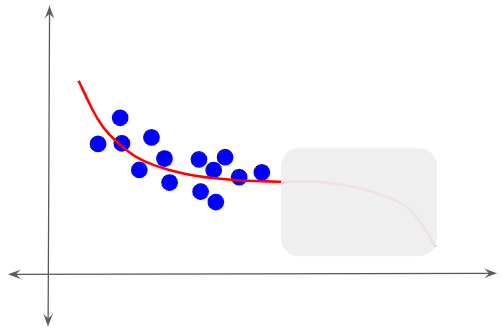
During training, each layer of the network learns an output function to fit its input. Let’s say that during one iteration, Layer ‘k’ receives a mini-batch of activations from the previous layer. It then adjusts its output activations by updating its weights based on that input.
However, in each iteration, the previous layer ‘k-1’ is also doing the same thing. It adjusts its output activations, effectively changing its distribution.
 How Covariate Shift affects Training (Image by Author)
That is also the input for layer ‘k’. In other words, that layer receives input data that has a different distribution than before. It is now forced to learn to fit to this new input. As we can see, each layer ends up trying to learn from a constantly shifting input, thus taking longer to converge and slowing down the training.
Therefore the proposed hypothesis was that Batch Norm helps to stabilize these shifting distributions from one iteration to the next, and thus speeds up training.
Theory 2 - Loss and Gradient Smoothening
The MIT paper published results that challenge the claim that addressing Covariate Shift is responsible for Batch Norm’s performance, and puts forward a different explanation.
In a typical neural network, the “loss landscape” is not a smooth convex surface. It is very bumpy with sharp cliffs and flat surfaces. This creates a challenge for gradient descent - because it could suddenly encounter an obstacle in what it thought was a promising direction to follow. To compensate for this, the learning rate is kept low so that we take only small steps in any direction.
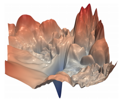 A neural network loss landscape (Source, by permission of Hao Li)
If you would like to read more about this, please see my article on neural network Optimizers that explains this in more detail, and how different Optimizer algorithms have evolved to tackle these challenges.
The paper proposes that what Batch Norm does is to smoothen the loss landscape substantially by changing the distribution of the network’s weights. This means that gradient descent can confidently take a step in a direction knowing that it will not find abrupt disruptions along the way. It can thus take larger steps by using a bigger learning rate.
To investigate this theory, the paper conducted an experiment to analyze the loss landscape of a model during training. We’ll try and visualize this with a simple example.
Let’s say that we have a simple network with two weight parameters (w1 and w2). The values of these weights can be shown on a 2D surface, with one axis for each weight. Each combination of weight values corresponds to a point on this 2D plane.
As the weights change during training, we move to another point on this surface. Hence one can plot the trajectory of the weights over the training iterations.
Note that the picture below displays only the weight values at each point. To visualize the loss, imagine a 3D surface, with a third axis for the loss coming out of the page. If we measured and plotted the loss for all the different combinations of weights, the shape of that loss curve is called the loss landscape.
 (Image by Author)
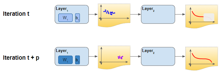
The goal of the experiment was to examine the loss landscape, by measuring what the Loss and Gradient would look like at different points if we kept moving in the same direction. They measured this with and without Batch Norm, to see what effect Batch Norm had.
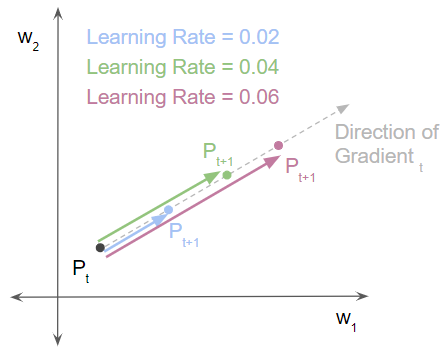
let’s say that at some iteration ‘t’ during training it is at point P(t). It evaluates the loss and the gradient at P(t). Then, starting from that point, it takes a single step forward with some learning rate to reach the next point P(t+1). Then it does a rewind back to Pt and repeats the step with a higher learning rate.
In other words, it tried three different alternatives by taking three different-sized steps (blue, green, and pink arrows) along the gradient direction, using three different learning rates. That brought us to three different next points for P(t+1). Then, at each of those P(t+1) points, it measured the new loss and gradient.
After this, it repeated all three steps for the same network, but with Batch Norm included.
- (Image by Author)*
Now we can plot the loss at each of those P(t+1) points (blue, green, and pink) just in that single direction. The bumpy red curve shows the loss without Batch Norm and the smooth declining yellow curve shows the loss with Batch Norm.
 Loss with Batch declines smoothly (Image by Author)
Similarly, we can plot the size and direction of the gradient at each of those points. The red arrows show the gradient fluctuating wildly in size and direction without Batch Norm. The yellow arrows show the gradient remaining steady in size and direction with Batch Norm.
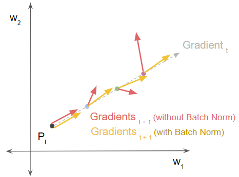 Gradients with Batch Norm are smoother (Image by Author)
This experiment shows us that Batch Norm significantly smoothens the loss landscape. How does that help our training?
The ideal scenario is that at the next point P_t+1, the gradient also lies in the same direction. This means that we can continue moving in the same direction. This allows the training to proceed smoothly and quickly find the minimum.
On the other hand, if the best gradient direction at P(t+1) took us in a different direction, we would end up following a zig-zag route with wasted effort. That would require more training iterations to converge.
Although this paper’s findings have not been challenged so far, it isn’t clear whether they’ve been fully accepted as conclusive proof to close this debate.
Regardless of which theory is correct, what we do know for sure is that Batch Norm provides several advantages.
Advantages of Batch Norm
The huge benefit that Batch Norm provides is to allow the model to converge faster and speed up training. It makes the training less sensitive to how the weights are initialized and to the precise tuning of hyperparameters.
Batch Norm lets you use higher learning rates. Without Batch Norm, learning rates have to be kept small to prevent large outlier gradients from affecting the gradient descent. Batch Norm helps to reduce the effect of these outliers.
Batch Norm also reduces the dependence of gradients on the initial weight values. Since weights are initialized randomly, outlier weight values in the early phases of training can distort gradients. Thus it takes longer for the network to converge. Batch Norm helps to dampen the effects of these outliers.
When is Batch Norm not applicable?
Batch Norm doesn’t work well with smaller batch sizes. That results in too much noise in the mean and variance of each mini-batch.
Batch Norm is not used with recurrent networks. Activations after each timestep have different distributions, making it impractical to apply Batch Norm to it.
Conclusion
Even though we aren’t sure about the correct explanation, it is fascinating to explore these different theories as it gives us some insight into the inner workings of neural networks.
Regardless, Batch Norm is a layer that we should definitely consider when designing our architecture.
And finally, if you liked this article, you might also enjoy my other series on Transformers, Audio Deep Learning, and Geolocation Machine Learning.
Let’s keep learning!