Batch Norm Explained Visually — How it works, and why neural networks need it

Batch Norm is an essential part of the toolkit of the modern deep learning practitioner. Soon after it was introduced in the Batch Normalization paper, it was recognized as being transformational in creating deeper neural networks that could be trained faster.

Batch Norm is a neural network layer that is now commonly used in many architectures. It often gets added as part of a Linear or Convolutional block and helps to stabilize the network during training.

In this article, we will explore what Batch Norm is, why we need it and how it works.

But before we talk about Batch Normalization itself, let’s start with some background about Normalization.

Normalizing Input Data

When inputting data to a deep learning model, it is standard practice to normalize the data to zero mean and unit variance. What does this mean and why do we do this?

Let’s say the input data consists of several features x1, x2,…xn. Each feature might have a different range of values. For instance, values for feature x1 might range from 1 through 5, while values for feature x2 might range from 1000 to 99999.

So, for each feature column separately, we take the values of all samples in the dataset and compute the mean and the variance. And then normalize the values using the formula below.

How we normalize (Image by Author)

In the picture below, we can see the effect of normalizing data. The original values (in blue) are now centered around zero (in red). This ensures that all the feature values are now on the same scale.

What normalized data looks like (Image by Author)

To understand what happens without normalization, let’s look at an example with just two features that are on drastically different scales. Since the network output is a linear combination of each feature vector, this means that the network learns weights for each feature that are also on different scales. Otherwise, the large feature will simply drown out the small feature.

Then during gradient descent, in order to “move the needle” for the Loss, the network would have to make a large update to one weight compared to the other weight. This can cause the gradient descent trajectory to oscillate back and forth along one dimension, thus taking more steps to reach the minimum.

Features on different scales take longer to reach the minimum (Image by Author)

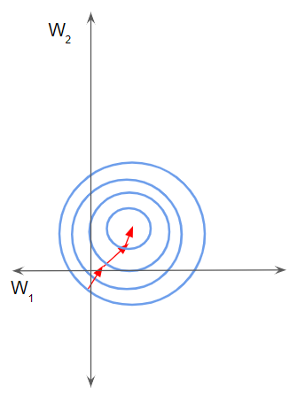
In this case, the loss landscape looks like a narrow ravine. We can decompose the gradient along the two dimensions. It is steep along one dimension and much more gentle along the other dimension.

We end up making a larger update to one weight due to its large gradient. This causes the gradient descent to bounce to the other side of the slope. On the other hand, the smaller gradient along the second direction results in us making smaller weight updates and thus taking smaller steps. This uneven trajectory takes longer for the network to converge.

A narrow valley causes gradient descent to bounce from one slope to the other (Image by Author)

Instead, if the features are on the same scale, the loss landscape is more uniform like a bowl. Gradient descent can then proceed smoothly down to the minimum.

Normalized data helps the network converge faster (Image by Author)

If you would like to read more about this, please see my article on neural network Optimizers that explains this in more detail, as well as how different Optimizer algorithms have evolved to tackle these challenges.

The need for Batch Norm

Now that we understand what Normalization is, the reason for needing Batch Normalization starts to become clear.

Consider any of the hidden layers of a network. The activations from the previous layer are simply the inputs to this layer. For instance, from the perspective of Layer 2 in the picture below, if we “blank out” all the previous layers, the activations coming from Layer 1 are no different from the original inputs.

The same logic that requires us to normalize the input for the first layer will also apply to each of these hidden layers.

The inputs of each hidden layer are the activations from the previous layer, and must also be normalized (Image by Author)

In other words, if we are able to somehow normalize the activations from each previous layer then the gradient descent will converge better during training. This is precisely what the Batch Norm layer does for us.

How Does Batch Norm work?

Batch Norm is just another network layer that gets inserted between a hidden layer and the next hidden layer. Its job is to take the outputs from the first hidden layer and normalize them before passing them on as the input of the next hidden layer.

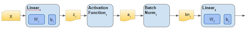The Batch Norm layer normalizes activations from Layer 1 before they reach layer 2 (Image by Author)

Just like the parameters (eg. weights, bias) of any network layer, a Batch Norm layer also has parameters of its own:

• Two learnable parameters called beta and gamma.
• Two non-learnable parameters (Mean Moving Average and Variance Moving Average) are saved as part of the ‘state’ of the Batch Norm layer.

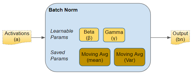Parameters of a Batch Norm layer (Image by Author)

These parameters are per Batch Norm layer. So if we have, say, three hidden layers and three Batch Norm layers in the network, we would have three learnable beta and gamma parameters for the three layers. Similarly for the Moving Average parameters.

Each Batch Norm layer has its own copy of the parameters (Image by Author)

During training, we feed the network one mini-batch of data at a time. During the forward pass, each layer of the network processes that mini-batch of data. The Batch Norm layer processes its data as follows:

1. The activations from the previous layer are passed as input to the Batch Norm. There is one activation vector for each feature in the data.
2. For each activation vector separately, calculate the mean and variance of all the values in the mini-batch.
3. Calculate the normalized values for each activation feature vector using the corresponding mean and variance. These normalized values now have zero mean and unit variance.

4. This step is the huge innovation introduced by Batch Norm that gives it its power. Unlike the input layer, which requires all normalized values to have zero mean and unit variance, Batch Norm allows its values to be shifted (to a different mean) and scaled (to a different variance). It does this by multiplying the normalized values by a factor, beta, and adding to it a factor, gamma. Note that this is an element-wise multiply, not a matrix multiply.

   What makes this innovation ingenious is that these factors are not hyperparameters (ie. constants provided by the model designer) but are trainable parameters that are learned by the network. In other words, each Batch Norm layer is able to optimally find the best factors for itself, and can thus shift and scale the normalized values to get the best predictions.

5. In addition, Batch Norm also keeps a running count of the Exponential Moving Average (EMA) of the mean and variance. During training, it simply calculates this EMA but does not do anything with it. At the end of training, it simply saves this value as part of the layer’s state, for use during the Inference phase. We will return to this point a little later when we talk about Inference. The Moving Average calculation uses a scalar ‘momentum’ denoted by alpha below. This is a hyperparameter that is used only for Batch Norm moving averages and should not be confused with the momentum that is used in the Optimizer.

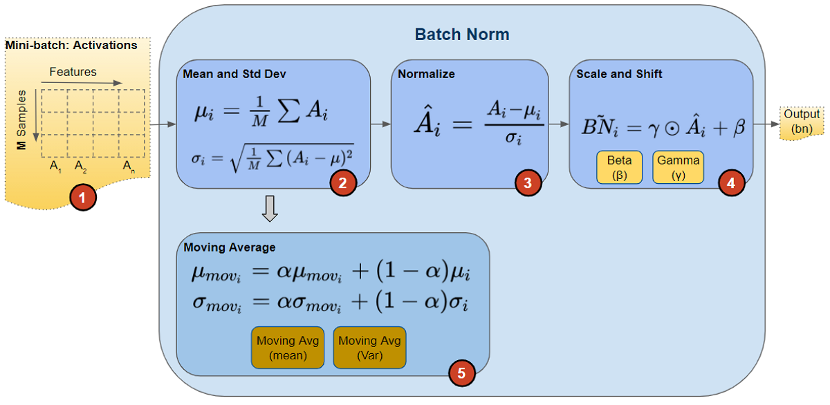Calculations performed by Batch Norm layer (Image by Author)

Below, we can see the shapes of these vectors. The values that are involved in computing the vectors for a particular feature are also highlighted in red. However, remember that all feature vectors are computed in a single matrix operation.

Shapes of Batch Norm vectors (Image by Author)

After the forward pass, we do the backward pass as normal. Gradients are calculated and updates are done for all layer weights, as well as for all beta and gamma parameters in the Batch Norm layers.

Batch Norm during Inference

As we discussed above, during Training, Batch Norm starts by calculating the mean and variance for a mini-batch. However, during Inference, we have a single sample, not a mini-batch. How do we obtain the mean and variance in that case?

Here is where the two Moving Average parameters come in - the ones that we calculated during training and saved with the model. We use those saved mean and variance values for the Batch Norm during Inference.

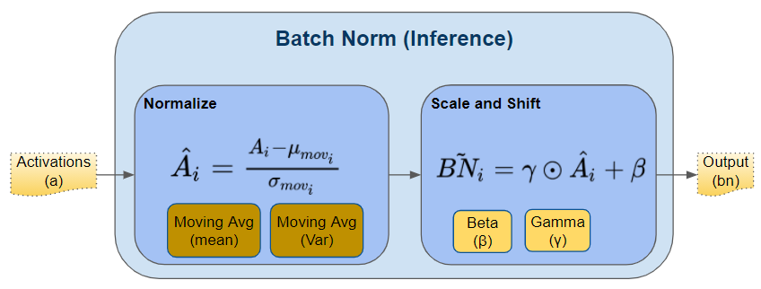Batch Norm calculation during Inference (Image by Author)

Ideally, during training, we could have calculated and saved the mean and variance for the full data. But that would be very expensive as we would have to keep values for the full dataset in memory during training. Instead, the Moving Average acts as a good proxy for the mean and variance of the data. It is much more efficient because the calculation is incremental - we have to remember only the most recent Moving Average.

Order of placement of Batch Norm layer

There are two opinions for where the Batch Norm layer should be placed in the architecture - before and after activation. The original paper placed it before, although I think you will find both options frequently mentioned in the literature. Some say ‘after’ gives better results.

Batch Norm can be used before or after activation (Image by Author)

Conclusion

Batch Norm is a very useful layer that you will end up using often in your network architecture. Hopefully, this gives you a good understanding of how Batch Norm works.

It is also useful to understand why Batch Norm helps in network training, which I will cover in detail in another article.

And finally, if you liked this article, you might also enjoy my other series on Transformers as well as Audio Deep Learning.

Let’s keep learning!