Foundations of NLP Explained Visually - Beam Search, How It Works

Many NLP applications such as machine translation, chatbots, text summarization, and language models generate some text as their output. In addition applications like image captioning or automatic speech recognition (ie. Speech-to-Text) output text, even though they may not be considered pure NLP applications.

There are a couple of commonly used algorithms used by all of these applications as part of their last step to produce their final output.

• Greedy Search is one such algorithm. It is used often because it is simple and quick.
• The alternative is to use Beam Search. It is very popular because, although it requires more computation, it usually produces much better results.

In this article, I will explore Beam Search and explain why it is used and how it works. We will briefly touch upon Greedy Search as a comparison so that we can understand how Beam Search improves upon it.

Also, if you are interested in NLP, I have a few more articles that you might find useful. They explore other fascinating topics in this space such as Transformers and Speech-to-Text.

1. Transformers Explained Visually: Overview of functionality (How Transformers are used, and why they are better than RNNs. Components of the architecture, and behavior during Training and Inference)
2. How Transformers work, step-by-step (Internal operation end-to-end. How data flows and what computations are performed, including matrix representations)
3. Automatic Speech Recognition (Speech-to-Text algorithm and architecture, using CTC Loss and Decoding for aligning sequences.)

We’ll start by getting some context regarding how NLP models generate their output so that we can understand where Beam Search (and Greedy Search) fits in.

NB: Depending on the problem they’re solving, NLP models can generate output as either characters or words. All of the concepts related to Beam Search apply equivalently to either, so I will use both terms interchangeably in this article.

How NLP models generate output

Let’s take a sequence-to-sequence model as an example. These models are frequently used for applications such as machine translation.

Sequence-to-Sequence Model for Machine Translation (Image by Author)

For instance, if this model were being used to translate from English to Spanish, it would take a sentence in the source language (eg. “You are welcome” in English) as input and output the equivalent sentence in the target language (eg. “De nada” in Spanish).

Text is a sequence of words (or characters), and the NLP model constructs a vocabulary consisting of the entire set of words in the source and target languages.

The model takes the source sentence as its input and passes it through an Embedding layer followed by an Encoder. The Encoder then outputs an encoded representation that compactly captures the essential features of the input.

This representation is then fed to a Decoder along with a “<START>” token to seed its output. The Decoder uses these to generate its own output, which is an encoded representation of the sentence in the target language.

This is then passed through an output layer, which might consist of some Linear layers followed by a Softmax. The Linear layers output a score of the likelihood of occurrence of each word in the vocabulary, at each position in the output sequence. The Softmax then converts those scores into probabilities.

Probabilities for each character in the vocabulary, for each position in the output sequence (Image by Author)

Our eventual goal, of course, is not these probabilities but a final target sentence. To get that, the model has to decide which word it should predict for each position in that target sequence.

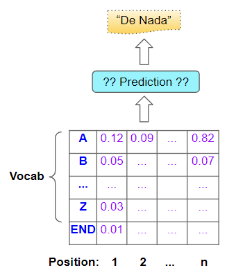The model predicts an output sentence based on the probabilities (Image by Author)

How does it do that?

Greedy Search

A fairly obvious way is to simply take the word that has the highest probability at each position and predict that. It is quick to compute and easy to understand, and often does produce the correct result.

Greedy Search (Image by Author)

In fact, Greedy Search is so easy to understand, that we don’t need to spend more time explaining it 😃. But can we do better?

Aha, finally that brings us to our real topic!

Beam Search

Beam Search makes two improvements over Greedy Search.

• With Greedy Search, we took just the single best word at each position. In contrast, Beam Search expands this and takes the best ’N’ words.
• With Greedy Search, we considered each position in isolation. Once we had identified the best word for that position, we did not examine what came before it (ie. in the previous position), or after it. In contrast, Beam Search picks the ’N’ best sequences so far and considers the probabilities of the combination of all of the preceding words along with the word in the current position.

In other words, it is casting the “light beam of its search” a little more broadly than Greedy Search, and this is what gives it its name. The hyperparameter ’N’ is known as the Beam width.

Intuitively it makes sense that this gives us better results over Greedy Search. Because, what we are really interested in is the best complete sentence, and we might miss that if we picked only the best individual word in each position.

Beam Search — What it does

Let’s take a simple example with a Beam width of 2, and using characters to keep it simple.

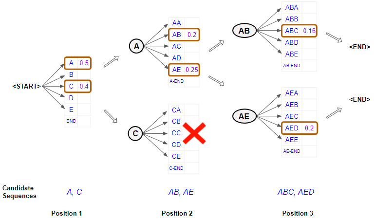Beam Search example, with width = 2 (Image by Author)

First Position

• Consider the output of the model at the first position. It starts with the “<START>” token and obtains probabilities for each word. It now selects the two best characters in that position. eg. “A” and “C”.

Second Position

• When it comes to the second position, it re-runs the model twice to generate probabilities by fixing the possible characters in the first position. In other words, it constrains the characters in the first position to be either an “A” or a “C” and generates two branches with two sets of probabilities. The branch with the first set of probabilities corresponds to having “A” in position 1, and the branch with the second set corresponds to having “C” in position 1.
• It now picks the overall two best character pairs based on the combined probability of the first two characters, from out of both sets of probabilities. So it doesn’t pick just one best character pair from the first set and one best character pair from the second set. eg. “AB” and “AE”

Third Position

• When it comes to the third position, it repeats the process. It re-runs the model twice by constraining the first two positions to be either “AB” or “AE” and again generates two sets of probabilities.
• Once more, it picks the overall two best character triplets based on the combined probability of the first three characters from both sets of probabilities. Therefore we now have the two best combinations of characters for the first three positions. eg. “ABC” and “AED”.

Repeat till END token

• It continues doing this till it picks an “<END>” token as the best character for some position, which then concludes that branch of the sequence.

It finally ends up with the two best sequences and predicts the one with the higher overall probability.

Beam Search — How it works

We now understand Beam Search at a conceptual level. Let’s go one level deeper and understand the details of how this works. We’ll continue with the same example and use a Beam width of 2.

Continuing with our sequence-to-sequence model, the Encoder and Decoder would likely be a recurrent network consisting of some LSTM layers. Alternately it could also be built using Transformers rather than a recurrent network.

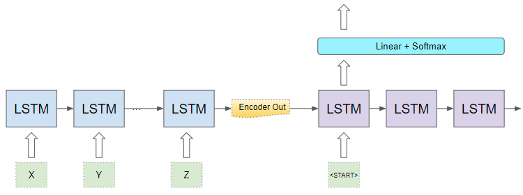An LSTM-based Sequence-to-Sequence model (Image by Author)

Let’s focus on the Decoder component and the output layers.

First Position

In the first timestep, it uses the Encoder’s output and an input of a “<START>” token to generate the character probabilities for the first position.

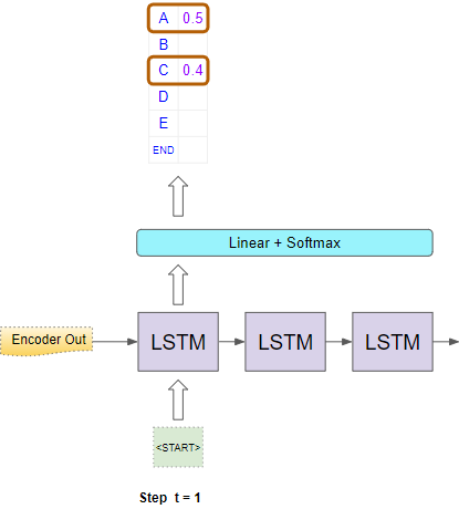Character probabilities for the first position (Image by Author)

Now it picks two characters with the highest probability eg. “A” and “C”.

Second Position

For the second timestep, it then runs the Decoder twice using the Encoder’s output as before. Along with the “<START>” token in the first position, it forces the input of the second position to be “A” in the first Decoder run. In the second Decoder run, it forces the input of the second position to be “C”.

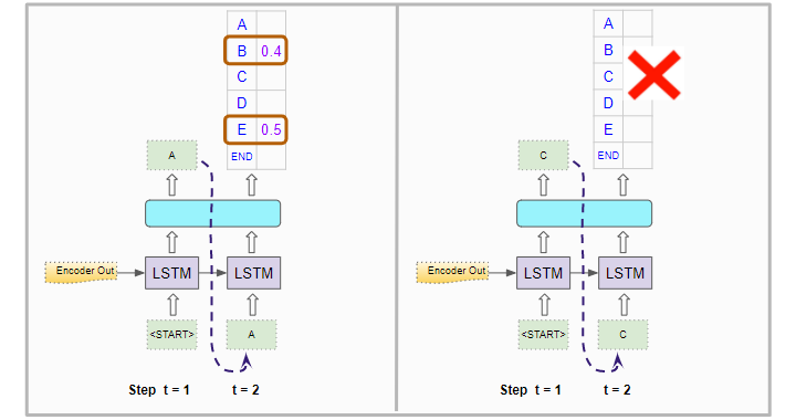Character probabilities for the second position (Image by Author)

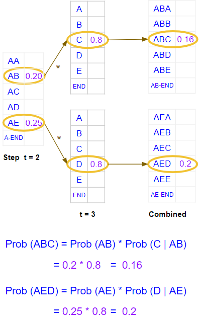
It generates character probabilities for the second position. But these are individual character probabilities. It needs to compute the combined probabilities for character pairs in the first two positions. The probability of the pair “AB” is the probability of “A” occurring in the first position multiplied by the probability of “B” occurring in the second position, given that “A” is already fixed in the first position. The example below shows the calculation.

Calculate probabilities for character-pairs in the first two positions (Image by Author)

It does this for both Decoder runs and picks the character pairs with the highest combined probabilities across both runs. It, therefore, picks “AB” and “AE”.

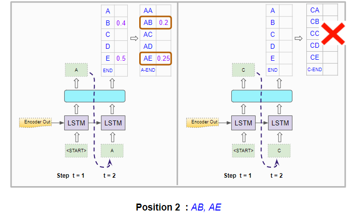The model picks the two best character pairs based on the combined probability (Image by Author)

Third Position

For the third time step, it again runs the Decoder twice as before. Along with the “<START>” token in the first position, it forces the input of the second position and third positions to be “A” and “B” respectively in the first Decoder run. In the second Decoder run, it forces the input of the second position and third positions to be “A” and “E” respectively.

Character probabilities for the third position (Image by Author)

It calculates the combined probability for character triples in the first three positions.

Calculate probabilities for character-triples in the first three positions (Image by Author)

It picks the two best ones across both runs, and therefore picks “ABC” and “AED”.

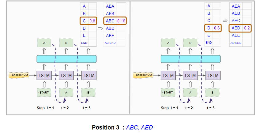The model picks the two best character triples based on the combined probability (Image by Author)

Repeat till END token

It repeats this process till it generates two best sequences that end with an “<END>” token.

It then chooses the sequence that has the highest combined probability to make its final prediction.

Conclusion

This gives us a sense of what Beam Search does, how it works, and why it gives us better results. This comes at the expense of increased computation, and longer execution times. So we should evaluate whether that tradeoff makes sense for our application’s use case.

And finally, if you liked this article, you might also enjoy my other series on Audio Deep Learning and Reinforcement Learning.

Audio Deep Learning Made Simple (Part 1): State-of-the-Art Techniques

Reinforcement Learning Made Simple (Part 1): Intro to Basic Concepts and Terminology

Let’s keep learning!