Audio Deep Learning Made Simple - State-of-the-Art Techniques

Although Computer Vision and NLP applications get most of the buzz, there are many groundbreaking use cases for deep learning with audio data that are transforming our daily lives. Over the next few articles, I aim to explore the fascinating world of audio deep learning.

Here’s a quick summary of the articles I am planning in the series. My goal throughout will be to understand not just how something works but why it works that way.

State-of-the-Art Techniques — this article (What is sound and how it is digitized. What problems is audio deep learning solving in our daily lives. What are Spectrograms and why they are all-important.)
Why Mel Spectrograms perform better (Processing audio data in Python. What are Mel Spectrograms and how to generate them)
Feature Optimization and Augmentation (Enhance Spectrograms features for optimal performance by hyper-parameter tuning and data augmentation)
Audio Classification (End-to-end example and architecture to classify ordinary sounds. Foundational application for a range of scenarios.)
Automatic Speech Recognition (Speech-to-Text algorithm and architecture, using CTC Loss and Decoding for aligning sequences.)

In this first article, since this area may not be as familiar to people, I will introduce the topic and provide an overview of the deep learning landscape for audio applications. We will understand what audio is and how it is represented digitally. I will talk about the wide-ranging impact that audio applications have on our daily lives, and explore the architecture and model techniques that they use.

What is sound?

We all remember from school that a sound signal is produced by variations in air pressure. We can measure the intensity of the pressure variations and plot those measurements over time.

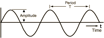
Sound signals often repeat at regular intervals so that each wave has the same shape. The height shows the intensity of the sound and is known as the amplitude.

Simple repeating signal showing Amplitude vs Time (by permission of Prof Mark Liberman)

The time taken for the signal to complete one full wave is the period. The number of waves made by the signal in one second is called the frequency. The frequency is the reciprocal of the period. The unit of frequency is Hertz.

The majority of sounds we encounter may not follow such simple and regular periodic patterns. But signals of different frequencies can be added together to create composite signals with more complex repeating patterns. All sounds that we hear, including our own human voice, consist of waveforms like these. For instance, this could be the sound of a musical instrument.

Musical waveform with a complex repeating signal (Source, by permission of Prof George Gibson)

The human ear is able to differentiate between different sounds based on the ‘quality’ of the sound which is also known as timbre.

How do we represent sound digitally?

To digitize a sound wave we must turn the signal into a series of numbers so that we can input it into our models. This is done by measuring the amplitude of the sound at fixed intervals of time.

Sample measurements at regular time intervals (Source)

Each such measurement is called a sample, and the sample rate is the number of samples per second. For instance, a common sampling rate is about 44,100 samples per second. That means that a 10-second music clip would have 441,000 samples!

Preparing audio data for a deep learning model

Till a few years ago, in the days before Deep Learning, machine learning applications of Computer Vision used to rely on traditional image processing techniques to do feature engineering. For instance, we would generate hand-crafted features using algorithms to detect corners, edges, and faces. With NLP applications as well, we would rely on techniques such as extracting N-grams and computing Term Frequency.

Similarly, audio machine learning applications used to depend on traditional digital signal processing techniques to extract features. For instance, to understand human speech, audio signals could be analyzed using phonetics concepts to extract elements like phonemes. All of this required a lot of domain-specific expertise to solve these problems and tune the system for better performance.

However, in recent years, as Deep Learning becomes more and more ubiquitous, it has seen tremendous success in handling audio as well. With deep learning, the traditional audio processing techniques are no longer needed, and we can rely on standard data preparation without requiring a lot of manual and custom generation of features.

What is more interesting is that, with deep learning, we don’t actually deal with audio data in its raw form. Instead, the common approach used is to convert the audio data into images and then use a standard CNN architecture to process those images! Really? Convert sound into pictures? That sounds like science fiction. 😄

The answer, of course, is fairly commonplace and mundane. This is done by generating Spectrograms from the audio. So first let’s learn what a Spectrum is, and use that to understand Spectrograms.

Spectrum

As we discussed earlier, signals of different frequencies can be added together to create composite signals, representing any sound that occurs in the real-world. This means that any signal consists of many distinct frequencies and can be expressed as the sum of those frequencies.

The Spectrum is the set of frequencies that are combined together to produce a signal. eg. the picture shows the spectrum of a piece of music.

The Spectrum plots all of the frequencies that are present in the signal along with the strength or amplitude of each frequency.

Spectrum showing the frequencies that make up a sound signal (Source, by permission of Prof Barry Truax)

The lowest frequency in a signal called the fundamental frequency. Frequencies that are whole number multiples of the fundamental frequency are known as harmonics.

For instance, if the fundamental frequency is 200 Hz, then its harmonic frequencies are 400 Hz, 600 Hz, and so on.

Time Domain vs Frequency Domain

The waveforms that we saw earlier showing Amplitude against Time are one way to represent a sound signal. Since the x-axis shows the range of time values of the signal, we are viewing the signal in the Time Domain.

The Spectrum is an alternate way to represent the same signal. It shows Amplitude against Frequency, and since the x-axis shows the range of frequency values of the signal, at a moment in time, we are viewing the signal in the Frequency Domain.

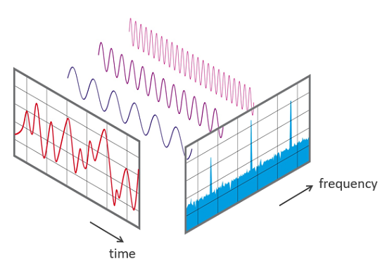Time Domain and Frequency Domain (Source)

Spectrograms

Since a signal produces different sounds as it varies over time, its constituent frequencies also vary with time. In other words, its Spectrum varies with time.

A Spectrogram of a signal plots its Spectrum over time and is like a ‘photograph’ of the signal. It plots Time on the x-axis and Frequency on the y-axis. It is as though we took the Spectrum again and again at different instances in time, and then joined them all together into a single plot.

It uses different colors to indicate the Amplitude or strength of each frequency. The brighter the color the higher the energy of the signal. Each vertical ‘slice’ of the Spectrogram is essentially the Spectrum of the signal at that instant in time and shows how the signal strength is distributed in every frequency found in the signal at that instant.

In the example below, the first picture displays the signal in the Time domain ie. Amplitude vs Time. It gives us a sense of how loud or quiet a clip is at any point in time, but it gives us very little information about which frequencies are present.

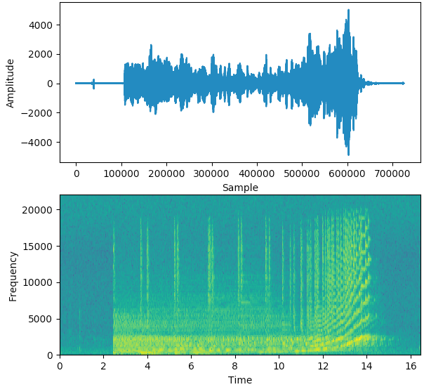Sound signal and its Spectrogram (Image by Author)

The second picture is the Spectrogram and displays the signal in the Frequency domain.

Generating Spectrograms

Spectrograms are produced using Fourier Transforms to decompose any signal into its constituent frequencies. If this makes you a little nervous because we have now forgotten all that we learned about Fourier Transforms during college, don’t worry 😄! We won’t actually need to recall all the mathematics, there are very convenient Python library functions that can generate spectrograms for us in a single step. We’ll see those in the next article.

Audio Deep Learning Models

Now that we understand what a Spectrogram is, we realize that it is an equivalent compact representation of an audio signal, somewhat like a ‘fingerprint’ of the signal. It is an elegant way to capture the essential features of audio data as an image.

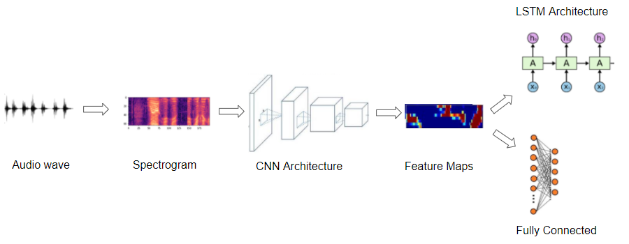Typical pipeline used by audio deep learning models (Image by Author)

So most deep learning audio applications use Spectrograms to represent audio. They usually follow a procedure like this:

Start with raw audio data in the form of a wave file.
Convert the audio data into its corresponding spectrogram.
Optionally, use simple audio processing techniques to augment the spectrogram data. (Some augmentation or cleaning can also be done on the raw audio data before the spectrogram conversion)
Now that we have image data, we can use standard CNN architectures to process them and extract feature maps that are an encoded representation of the spectrogram image.

The next step is to generate output predictions from this encoded representation, depending on the problem that you are trying to solve.

For instance, for an audio classification problem, you would pass this through a Classifier usually consisting of some fully connected Linear layers.
For a Speech-to-Text problem, you could pass it through some RNN layers to extract text sentences from this encoded representation.

Of course, we are skipping many details, and making some broad generalizations, but in this article, we are staying at a fairly high-level. In the following articles, we’ll go into a lot more specifics about all of these steps and the architectures that are used.

What problems does audio deep learning solve?

Audio data in day-to-day life can come in innumerable forms such as human speech, music, animal voices, and other natural sounds as well as man-made sounds from human activity such as cars and machinery.

Given the prevalence of sounds in our lives and the range of sound types, it is not surprising that there are a vast number of usage scenarios that require us to process and analyze audio. Now that deep learning has come of age, it can be applied to solve a number of use cases.

Audio Classification

This is one of the most common use cases and involves taking a sound and assigning it to one of several classes. For instance, the task could be to identify the type or source of the sound. eg. is this a car starting, is this a hammer, a whistle, or a dog barking.

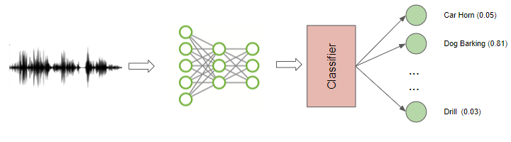Classification of Ordinary sounds (Image by Author)

Obviously, the possible applications are vast. This could be applied to detect the failure of machinery or equipment based on the sound that it produces, or in a surveillance system, to detect security break-ins.

Audio Separation and Segmentation

Audio Separation involves isolating a signal of interest from a mixture of signals so that it can then be used for further processing. For instance, you might want to separate out individual people’s voices from a lot of background noise, or the sound of the violin from the rest of the musical performance.

Separating individual speakers from a video (Source, by permission of Ariel Ephrat)

Audio Segmentation is used to highlight relevant sections from the audio stream. For instance, it could be used for diagnostic purposes to detect the different sounds of the human heart and detect anomalies.

Music Genre Classification and Tagging

With the popularity of music streaming services, another common application that most of us are familiar with is to identify and categorize music based on the audio. The content of the music is analyzed to figure out the genre to which it belongs. This is a multi-label classification problem because a given piece of music might fall under more than one genre. eg. rock, pop, jazz, salsa, instrumental as well as other facets such as ‘oldies’, ‘female vocalist’, ‘happy’, ‘party music’ and so on.

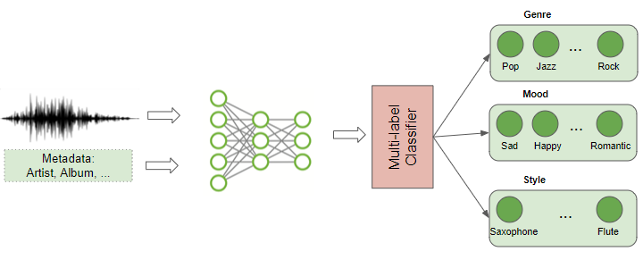Music Genre Classification and Tagging (Image by Author)

Of course, in addition to the audio itself, there is metadata about the music such as singer, release date, composer, lyrics and so on which would be used to add a rich set of tags to music.

This can be used to index music collections according to their audio features, to provide music recommendations based on a user’s preferences, or for searching and retrieving a song that is similar to a song to which you are listening.

Music Generation and Music Transcription

We have seen a lot of news these days about deep learning being used to programmatically generate extremely authentic-looking pictures of faces and other scenes, as well as being able to write grammatically correct and intelligent letters or news articles.

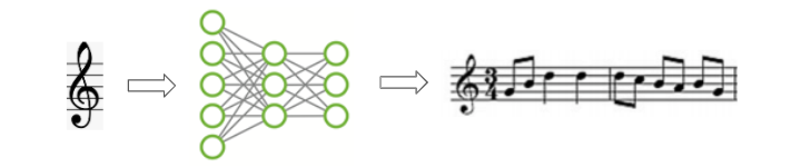Music Generation (Image by Author)

Similarly, we are now able to generate synthetic music that matches a particular genre, instrument, or even a given composer’s style.

In a way, Music Transcription applies this capability in reverse. It takes some acoustics and annotates it, to create a music sheet containing the musical notes that are present in the music.

Voice Recognition

Technically this is also a classification problem but deals with recognizing spoken sounds. It could be used to identify the gender of a speaker, or their name (eg. is this Bill Gates or Tom Hanks, or is this Ketan’s voice vs an intruder’s)

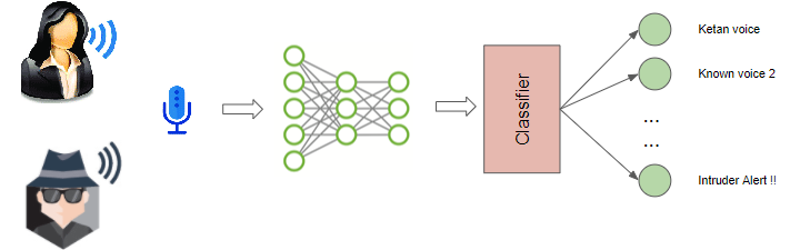Voice Recognition for Intruder Detection (Image by Author)

We might want to detect human emotion and identify the mood of the person from the tone of their voice eg. is the person happy, sad, angry, or stressed. We could apply this to animal voices to identify the type of animal that is producing a sound, or potentially to identify whether it is a gentle affectionate purring sound, a threatening bark, or a frightened yelp.

Speech to Text and Text to Speech

When dealing with human speech, we can go a step further, and not just recognize the speaker, but understand what they are saying. This involves extracting the words from the audio, in the language in which it is spoken and transcribing it into text sentences.

This is one of the most challenging applications because it deals not just with analyzing audio, but also with NLP and requires developing some basic language capability to decipher distinct words from the uttered sounds.

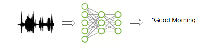Speech to Text (Image by Author)

Conversely, with Speech Synthesis, one could go in the other direction and take written text and generate speech from it, using, for instance, an artificial voice for conversational agents.

Being able to understand human speech obviously enables a huge number of useful applications both in our business and personal lives, and we are only just beginning to scratch the surface.

The most well-known examples that have achieved widespread use are virtual assistants like Alexa, Siri, Cortana, and Google Home, which are consumer-friendly products built around this capability.

Conclusion

In this article, we have stayed at a fairly high-level and explored the breadth of audio applications, and covered the general techniques applied to solve those problems.

In the next article, we will go into more of the technical details of pre-processing audio data and generating spectrograms. We will take a look at the hyperparameters that are used to tune performance.

That will then prepare us for delving deeper into a couple of end-to-end examples, starting with the Classification of ordinary sounds and culminating with the much more challenging Automatic Speech Recognition, where we will also cover the fascinating CTC algorithm.

And finally, if you liked this article, you might also enjoy my other series on Transformers as well as Reinforcement Learning.

Transformers Explained Visually: Overview of functionality

Reinforcement Learning Made Simple (Part 1): Intro to Basic Concepts and Terminology

Let’s keep learning!