Reinforcement Learning Made Simple - Intro to Basic Concepts and Terminology

You’ve probably started hearing a lot more about Reinforcement Learning in the last few years, ever since the AlphaGo model, which was trained using reinforcement-learning, stunned the world by beating the then reigning world champion at the complex game of Go.

Over a series of articles, I’ll go over the basics of Reinforcement Learning (RL) and some of the most popular algorithms and deep learning architectures used to solve RL problems. We’ll try to focus on understanding these principles in as intuitive a way as possible without going too much into mathematical theory.

Here’s a quick summary of the articles in the series. My goal throughout will be to understand not just how something works but why it works that way.

1. Intro to Basic Concepts and Terminology — this article (What is an RL problem, and how to apply an RL problem-solving framework to it using techniques from Markov Decision Processes and concepts such as Return, Value, and Policy)
2. Solution Approaches (Overview of popular RL solutions, and categorizing them based on the relationship between these solutions. Important takeaways from the Bellman equation, which is the foundation for all RL algorithms.)
3. Model-free algorithms (Similarities and differences of Value-based and Policy-based solutions using an iterative algorithm to incrementally improve predictions. Exploitation, Exploration, and ε-greedy policies.)
4. Q-Learning (In-depth analysis of this algorithm, which is the basis for subsequent deep-learning approaches. Develop intuition about why this algorithm converges to the optimal values.)
5. Deep Q Networks (Our first deep-learning algorithm. A step-by-step walkthrough of exactly how it works, and why those architectural choices were made.)
6. Policy Gradient (Our first policy-based deep-learning algorithm.)
7. Actor-Critic (Sophisticated deep-learning algorithm which combines the best of Deep Q Networks and Policy Gradients.)

Overview of RL

Where does RL fit in the world of Machine Learning?

Typically when people provide an overview of ML, the first thing they explain is that it can be divided into two categories, Supervised Learning and Unsupervised Learning. However, there is a third category, viz. RL although it isn’t mentioned as often as its two more glamorous siblings.

Machine Learning can be categorized as Supervised Learning, Unsupervised Learning and Reinforcement Learning (Image by Author)

Supervised Learning uses labeled data as input, and predicts outcomes. It receives feedback from a Loss function acting as a ‘supervisor’.

Unsupervised Learning uses unlabeled data as input and detects hidden patterns in the data such as clusters or anomalies. It receives no feedback from a supervisor.

Reinforcement Learning gathers inputs and receives feedback by interacting with the external world. It outputs the best actions that it needs to take while interacting with that world.

How is RL different from Supervised (or Unsupervised) Learning?

• There is no supervisor to guide the training
• You don’t train with a large (labeled or unlabeled) pre-collected dataset. Rather, your ‘data’ is provided to you dynamically via feedback from the real-world environment with which you are interacting.
• You iteratively make decisions over a sequence of time-steps eg. In a Classification problem, you run inference once on data input to produce an output prediction. With Reinforcement Learning, you run inference repeatedly, navigating through the real-world environment as you go.

What problems are RL used to solve?

Rather than the typical ML problems such as Classification, Regression, Clustering and so on, RL is most commonly used to solve a different class of real-world problems, such as a Control task or Decision task, where you operate a system that interacts with the real world.

• eg. A robot or drone that has to learn the task of picking a device from one box and putting it in a container

It is useful for a variety of applications like:

• Operating a drone or autonomous vehicle
• Manipulating a robot to navigate the environment and perform various tasks
• Managing an investment portfolio and taking trading decisions
• Playing games such as Go, Chess, video games

Reinforcement Learning happens through trial and error

With RL the learning happens from experience by trial and error, similar to a human eg. A baby can touch fire or milk and then learns from negative or positive reinforcement.

• The baby takes some action
• Receives feedback from the environment about the result of that action
• Repeats this process till it learns which actions produce favorable results and which actions produce unfavorable results.

A baby learns from positive and negative reinforcement (Image by Author)

To use RL, structure your problem as a Markov Decision Process

Let’s say you want to train a robot. How would you use RL to solve a problem like this?

To apply RL, the first step is to structure the problem as something called a Markov Decision Process (MDP). If you haven’t worked with RL before, chances are that the only thing you know about an MDP is that it sounds scary 😄.

So let’s try to understand what an MDP is. An MDP has five components that work together in a well-defined way.

Agent: it’s the system that you operate eg. the robot. This is the model that you want to build and train using RL.

Environment: the real-world environment with which the agent interacts as part of its operation. eg. The terrain that the robot has to navigate, its surroundings, factors such as wind, friction, lighting, temperature and so on.

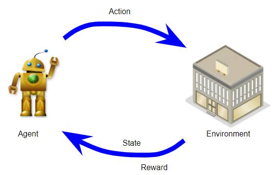An MDP has an Agent, Environment, States, Actions and Rewards (Image by Author)

State: this represents the current ‘state of the world’ at any point. eg. it could capture the position of the robot relative to its terrain, the position of objects around it, and perhaps the direction and speed of the wind.

There could be a finite or infinite set of states.

Action: these are the actions that the agent takes to interact with the environment. eg. The robot can turn right, left, move forward, go backward, bend, raise its hand and so on.

There could be a finite or infinite set of possible actions.

Reward: is the positive or negative reinforcement that the agent receives from the environment as a result of its actions. It is a way to evaluate the ‘good-ness’ or ‘bad-ness’ of a particular action.

eg. If moving in a particular direction causes the robot to run into a wall, that would have a negative reward. On the other hand, if turning left causes the robot to locate the object it needs to pick up, it would get a positive reward.

What should you keep in mind when defining your MDP?

Agent and Environment: Obviously, the first step is to decide the role and scope of your agent and the environment for the problem you are trying to solve.

State: Next, you have to define what data points the state contains and how they are represented.

The important thing is that it captures everything that is needed for your problem to represent the current world situation so that the agent can reason about the future without requiring information about the past or any additional knowledge.

In other words, the definition of the state should be self-contained. So, for instance, if you need to know something about how you arrived at this state, that history should be encapsulated within your state definition itself.

Actions: What is the set of the potential actions your agent can take?

Reward: This is how the agent learns from experience. So this is something that you need to give a fair amount of thought to because it is critical that you define the rewards in a way that truly reflects the behavior that you want your agent to learn.

How does an MDP work?

Now that we’ve seen what an MDP is, we’ll go into how it works. Let’s use the game of Tic-Tac-Toe (aka Noughts and Crosses) as a simple example. Two players play this game by placing their tokens on a 3x3 grid. One player places Noughts (the donut-shape) while the other places Crosses. The objective is to win the game by placing three of your tokens in a line.

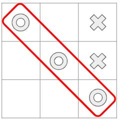(Image by Author)

You can define your MDP as follows:

• The agent plays against the environment, so the environment acts as its opponent.
• The state at any point, is the current position of all the tokens, both the agent’s and the environment’s, on the board.
• There are 9 possible actions where the agent can place its token at each of the 9 available squares in the grid.
• If the agent wins it gets a positive reward of +10 points and if it loses it gets a negative reward of -10 points. Each intermediate move gives a neutral reward of 0 points.

Now let’s go through the operation of the MDP as it plays the game.

The agent interacts with its environment over a sequence of time-steps. A set flow of operations occurs in each time-step and that flow then repeats in each time-step.

The sequence starts with an initial state, which becomes the current state. For instance, your opponent, the environment has placed their token in a particular position, and that is the starting state for the game.

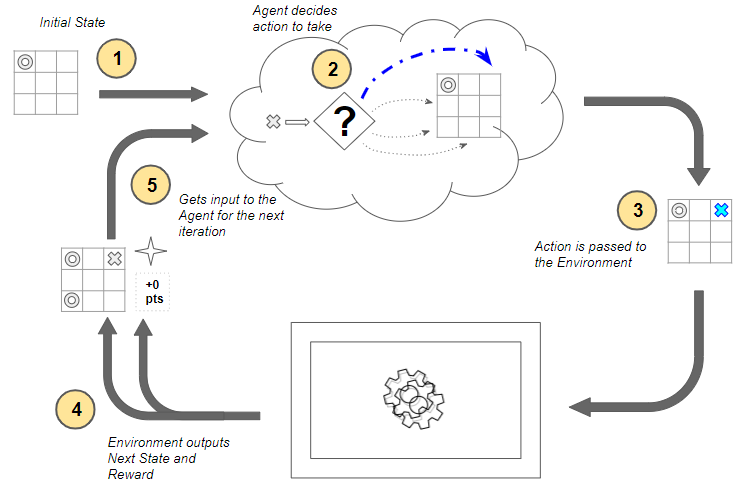How the MDP works (Image by Author)

Now, starting with the first time-step, the following steps occur at each time-step:

1. The environment’s current state is input to the agent.
2. The agent uses that current state to decide what action it should take. It does not need a memory of the full history of states and actions that came before it. The agent decides to place its token in some position. There are many possible actions to choose from, so how does it decide what action to take? It’s a very important question but we’ll come to that later.
3. That action is passed as input to the environment.
4. The environment uses the current state and the selected action and outputs two things — it transitions the world to the next state, and it provides some reward. For instance, it takes the next move by placing its token in some position and provides us a reward. In this case, since no one has won the game yet, it provides a neutral reward of 0 points. How the environment does this is opaque to the agent, and not in our control.
5. This reward from the environment is then provided as feedback to the agent as a consequence of the previous action. This completes one time-step and moves us to the next time-step. This next state now becomes the current state which is then provided to the agent as input, and the cycle repeats.

Throughout this process, it is the agent’s goal to maximize the total amount of rewards that it receives from taking actions in given states. It wants to maximize not just the immediate reward, but the cumulative rewards it receives over time. We will return to this topic shortly.

An MDP iterates over a sequence of time-steps

Here is another view of the MDP’s operation which shows the progression of time-steps.

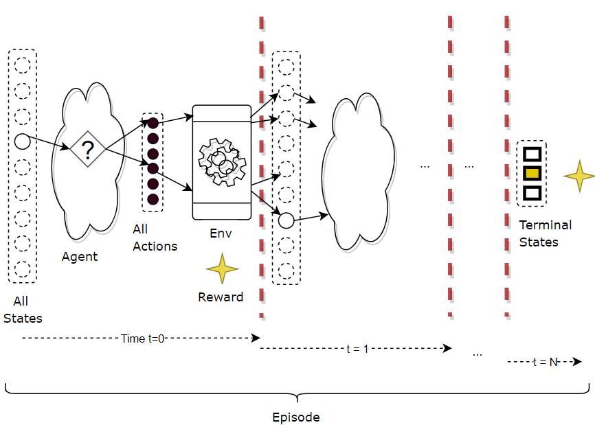An MDP iterates over a sequence of time steps (Image by Author)

In each time-step, three things occur — state, action and reward, which fully describe what happened in that time-step.

A Trajectory describes the execution over multiple time-steps

So the execution of the MDP can be described as a trajectory of occurrences (in terms of state, action, reward) over a sequence of time-steps, as below.

(s3,a3,r4, s4,a4,r5, s5,a5,r6, s6)

Episodic Tasks end in a Terminal State

For RL tasks that have a well-defined end or Terminal state, a complete sequence from the starting state to the end state is called an episode. eg. Each round of a game is an episode.

• So at the end of an episode, you can reset to a starting state (or randomly pick one from a set of starting states) and play another complete episode, and repeat.
• Each episode is independent of the next one.

Therefore an RL system’s operation repeats over multiple episodes. Within each episode, it repeats over multiple time-steps.

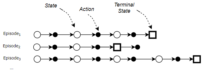Each Episode ends in a Terminal State (Image by Author)

Continuing Tasks go on forever

On the other hand, RL tasks which have no end are known as Continuing Tasks, and can go on forever (or till you stop the system). Eg. A robot that continuously manages manufacturing or warehouse automation.

Agent and Environment control the state-action transitions

As we just saw, the MDP operates by alternating between the agent doing something and then the environment doing something, in each time-step:

Given a state, the Agent decides the action. Given an action (and state), the Environment decides the next state. (Image by Author)

• Given the current state, the next action is decided by the agent. In fact, that is the only job of the agent. For instance, from the current state, the agent can choose, say, action a₁ or a₂ to place its token.
• Given the current state, and the next action chosen by the agent, the transition to the next state and the reward is controlled by the environment. For instance, if the agent had chosen action a₁, the environment could transition to state S₂ or S₃ by playing different moves. Another video game example could be that starting from a given state (eg. character is standing on a roof), the same agent action (character jumps) could with some probability, end up in more than one next state (eg. land on a neighboring roof, or fall to the ground), as controlled by the environment.

How does the environment transition to the next state?

Given a current state, and the action picked by the agent, how does the environment figure out the outcome ie. the next state and reward?

For most realistic RL problems that we will deal with, the answer will usually be that ‘it just does’. Most environments have complex internal dynamics that control how they behave when an action is taken from a particular state.

For instance, in a stock-trading RL application, the stock market environment has a range of unseen factors that determine how stock prices move. Or the environment in a drone navigation RL application depends on the laws of physics that control air flows, motion, thermodynamics, visibility and so on in a variety of terrains and micro-weather conditions.

Our focus is on training the agent and we can usually treat the environment as an external black box.

Note that this external black box might be a simulator for the environment. In many cases, it might not be practical to build a simulator and we would interact with the real environment directly.

However, just for completeness, let me briefly mention that if we did build such an environment model, an MDP would represent it as a large transition probability matrix or function.

(Image by Author)

This matrix maps a given state and action pair to:

• The next state, with some probability, since we could end up in different states each with some probability. This is known as the Transition Probability.
• The reward.

How does the Agent pick the action?

On the other hand, we are very interested in how the agent decides what action to pick in a given state. That is, in fact, precisely the RL problem that we want to solve.

For that it uses three concepts, which we will explore next:

• Return
• Policy
• Value

The Return is the total reward over all time-steps

As the agent executes time-steps, it accumulates reward at each time-step. However, rather than any individual reward, what we really care about is the cumulative rewards.

We call this the Return. It is the total reward that the agent accumulates over the duration of a task.

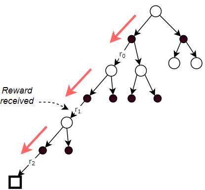The Return is the total of the rewards received at each time-step (Image by Author)

Return is computed using Discounted Rewards

When we calculate Return, rather than simply adding up all the rewards, we apply a discount factor γ to weight later rewards over time. These are known as Discounted Rewards.

Return = r₀ +γ r₁ + γ² r₂

and, more generally:

Return = r₀ +γ r₁ + γ² r₂ + ….+ γⁿ rₙ

This way, cumulative rewards do not grow infinitely as the number of time-steps becomes very large (like for continuing tasks, or for very long episodes).

It also encourages the agent to care more about the immediate reward compared to later rewards since later rewards will be more heavily discounted.

The ultimate goal of the agent is to get the maximum Return, not just over one episode, but over many, many episodes.

Based on this discount, we can see that there are two factors the agent considers when evaluating rewards.

Immediate Reward is more valuable than Later Reward

The first point is that if the agent had to choose between getting some amount of reward now versus later, the immediate reward is more valuable. Since the discount factor, γ, is less than 1, we will discount later rewards more than immediate rewards.

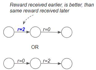Immediate Reward is more valuable than Later Reward (Image by Author)

Rewards that give us the highest Total Returns are better

The second point is that if the agent had to choose between getting some reward now versus getting a much bigger reward later, the bigger reward is most likely preferable. This is because we want the agent to look at total Returns rather than individual rewards. eg. In a game of chess, the agent has to pick the better of two paths. In the first, it can kill off a few pieces early on by playing aggressively. That gives it some immediate reward. However in the long run that puts it in a disadvantaged position, and it loses the game. Hence it gets a large negative reward at the end. Alternately it can play a different set of moves which yields lower rewards at first but where it ultimately wins the game. And thus gets a large positive reward. Clearly, the second approach is better since it gives a higher total Return as opposed to a bigger immediate reward.

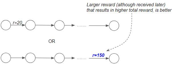We want to get a higher Total Reward (Image by Author)

Policy is the strategy followed to pick an action

The second concept for us to cover is Policy. Earlier we had deferred one very important question, which was, how the agent decides which action to pick in a given state. There can be many different strategies that an agent might use:

• Eg. Always pick the next action at random
• Eg. Always pick the next state that gives the highest known reward
• Eg. Take chances and explore new states in the hope of finding a better path.
• Eg. Always play it safe and avoid the chance of a negative reward.

Any strategy that the agent follows to decide which action to pick in a given state, is called a Policy. Although that sounds abstract, a Policy is simply something that maps a given state to an action to be taken.

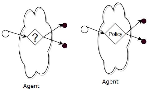The Policy tells the Agent which action to pick from any state (Image by Author)

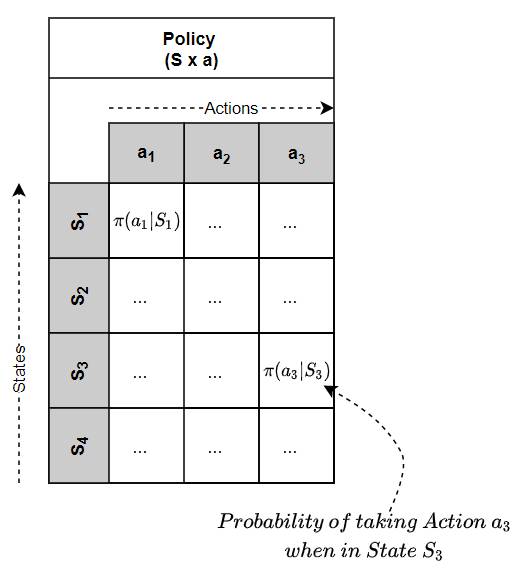
Policy is like a (huge) Lookup Table

You could think of a Policy as a (huge) Lookup Table which maps a state to an action.

(Image by Author)

So given the current state, the agent looks up that state in the table to find the action that it should pick.

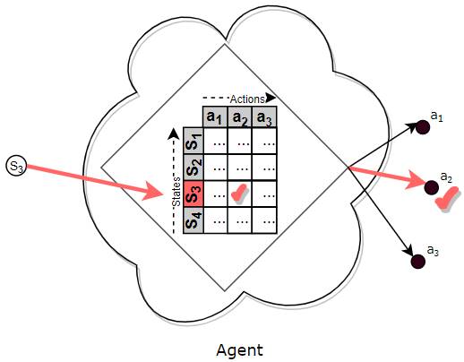The Policy is like a (huge) Lookup Table (Image by Author)

In practice, for real-world problems, there are so many states and so many actions, that a function is used, not a Lookup Table, that maps a state to an action.

However, the intuition is the same — think of a function as a ‘huge lookup table’.

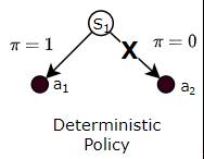
Deterministic and Stochastic Policies

Policies can be either Deterministic or Stochastic.

A Deterministic Policy is a Policy where the agent always chooses the same fixed action when it reaches a particular state.

(Image by Author)

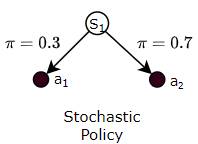
Alternately, a Stochastic Policy is a Policy where the agent varies the actions it chooses for a state, based on some probability for each action.

It might do this while playing a game, for instance, so that it doesn’t become completely predictable. Eg while playing Rock Paper Scissors, if it always played the same move, opponents can figure this out and easily defeat it.

(Image by Author)

How does the agent get a Policy?

We’ve been talking about the Policy as though the agent already had one readily available for it to use. But that is not really the case.

Much like a human baby, the agent doesn’t really have a useful policy when it starts out and has no idea what action it should take from any given state. Then, by using the Reinforcement Learning algorithm, it slowly learns a helpful policy that it can use.

There are so many possible Policies, which one should the Agent use?

The action that the agent takes from a given state determines the reward it obtains, and therefore over time, the eventual total Return. Hence the goal of the agent is to pick the action that maximizes its Return.

Put another way, the agent’s goal is to follow a Policy (which is how it picks its actions) that maximizes its Return.

So, out of all the Policies the agent could follow, it wants to pick the best one ie. the one which gives it the highest Return.

In order to do that, the agent needs to compare two Policies to decide which is better. For that, we need to understand the notion of Value.

The Value tells you the expected Return by following some Policy

Let’s say the agent is in a particular state. Also, let’s say that the agent has somehow been given a policy, π. Now, if it starts from that state, and always picks actions based on that policy, what is the Return it could expect to get?

This is the same as saying, if the agent starts from that state, and always picks actions based on that policy, what would its average Return be over many, many episodes?

This average long-term Return, or expected Return, is known as the Value of that particular state, under policy π.

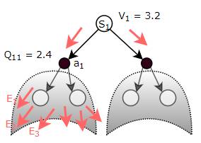The State Value (V) or the State-Action Value (Q) is the expected Return obtained from a particular state or state-action respectively, by following the given Policy over many episodes (Image by Author)

Alternately, the agent could start from a state-action pair ie. it has already taken a particular action from a particular state. If going forward from that state-action, it always picks actions based on the given policy π, what is the Return it could expect to get?

As discussed earlier for the Policy Table, we can think of Value as a (huge) Lookup Table which maps a State, or a State-Action pair, to a Value.

Thus we have two types of Value:

• State Value — the expected Return from a given state, by executing actions based on a given policy π from that state onward. In other words, the State Value function maps a State to its Value.

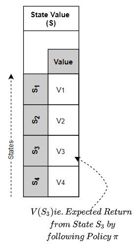The State Value Function maps a State to its Value (Image by Author)

• State-Action Value (aka Q-Value) — the expected Return by taking a given action from a given state, and then, by executing actions based on a given policy π after that. In other words, the State-Action Value function maps a State-Action pair to its Value.

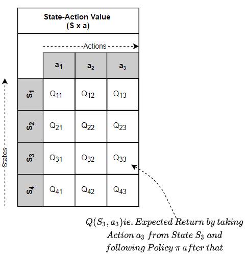The State-Action Value Function maps a State-Action pair to its Value (Image by Author)

Relationship between Reward, Return and Value

• Reward is the immediate reward obtained for a single action.
• Return is the total of all the discounted rewards obtained till the end of that episode.
• Value is the mean Return (aka expected Return) over many episodes.

Think of Reward as immediate pleasure and Value as long-lasting happiness 😃.

Intuitively one can think of Value as follows. Like a human, the agent learns from experience. As it interacts with the environment and completes episodes, it obtains the Returns for each episode.

As it accumulates more experience (ie. obtains Returns for more and more episodes), it gets a sense of which states, and which actions in those states yield the most Return.

It stores this ‘experience’ as ‘Value’.

Why does the Value depend on the policy we’re following?

Clearly, the rewards we get (and hence the Return and therefore the Value) depends on the action we take from a given state. And since the action depends on the chosen Policy, it follows that the Value depends on the Policy.

Eg. if our policy was to choose entirely random actions (i.e., sample actions from a uniform distribution), the Value (expected reward) of a state would probably be pretty low, since we’re definitely not choosing the best possible actions.

Eg. Instead, if our policy was to choose actions from a probability distribution that produces the maximum rewards when sampled, the Value (expected reward) of a state would be much higher.

Use the Value Function to compare Policies

Now that we understand Value, let’s go back to our earlier discussion about comparing two policies to see which is better. How do we evaluate what ’better’ means?

Given two policies, we can determine the corresponding State-Value or State-Action Value functions for each of those policies, by following the policy and evaluating the Returns.

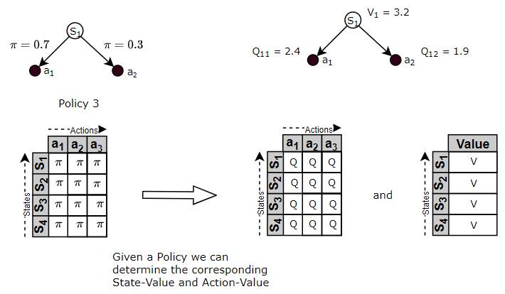(Image by Author)

Once we have the respective Value Functions, we can use those Value Functions to compare the policies. The policy, whose Value Function is higher, is better because that means it will yield higher Returns.

The ‘best’ Policy is called the Optimal Policy

Since we can now compare policies to figure out which ones are ‘good’ and which ones are ‘bad’, we can also use that to find the ‘best’ policy. This is known as the Optimal Policy.

The Optimal Policy is the policy that will yield more Returns to the agent than all other policies.

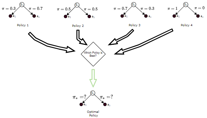The Optimal Policy is the one that is better than all other policies (Image by Author)

Solve the RL Problem by Finding the Optimal Policy

So now we have the approach to solve an RL problem.

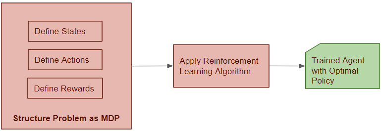
We structure our problem as an MDP and we can then solve this problem by building an agent viz. the brains of the MDP, in such a way that it can make decisions about which action to take. It should do this in a way that maximizes Returns.

In other words, we need to find the Optimal Policy for the agent. Once it has the Optimal Policy it simply uses that policy to pick actions from any state.

We will apply a Reinforcement Learning algorithm to build an agent model and train it to find the Optimal Policy. Finding the Optimal Policy essentially solves the RL problem.

(Image by Author)

In the next article in this series, we will look at the solution approach used by these RL algorithms.

And finally, if you liked this article, you might also enjoy my other series on Transformers as well as Audio Deep Learning.

Transformers Explained Visually - Overview of functionality

Audio Deep Learning Made Simple - State-of-the-Art Techniques

Let’s keep learning!