Audio Deep Learning Made Simple - Automatic Speech Recognition (ASR), How it Works

Over the last few years, Voice Assistants have become ubiquitous with the popularity of Google Home, Amazon Echo, Siri, Cortana, and others. These are the most well-known examples of Automatic Speech Recognition (ASR). This class of applications starts with a clip of spoken audio in some language and extracts the words that were spoken, as text. For this reason, they are also known as Speech-to-Text algorithms.

Of course, applications like Siri and the others mentioned above, go further. Not only do they extract the text but they also interpret and understand the semantic meaning of what was spoken, so that they can respond with answers, or take actions based on the user’s commands.

In this article, I will focus on the core capability of Speech-to-Text using deep learning. My goal throughout will be to understand not just how something works but why it works that way.

I have a few more articles in my audio deep learning series that you might find useful. They explore other fascinating topics in this space including how we prepare audio data for deep learning, why we use Mel Spectrograms for deep learning models and how they are generated and optimized.

1. State-of-the-Art Techniques (What is sound and how it is digitized. What problems is audio deep learning solving in our daily lives. What are Spectrograms and why they are all-important.)
2. Why Mel Spectrograms perform better (Processing audio data in Python. What are Mel Spectrograms and how to generate them)
3. Feature Optimization and Augmentation (Enhance Spectrograms features for optimal performance by hyper-parameter tuning and data augmentation)
4. Audio Classification (End-to-end example and architecture to classify ordinary sounds. Foundational application for a range of scenarios.)
5. Automatic Speech Recognition — this article (Speech-to-Text algorithm and architecture, using CTC Loss and Decoding for aligning sequences.)

Speech-to-Text

As we can imagine, human speech is fundamental to our daily personal and business lives, and Speech-to-Text functionality has a huge number of applications. One could use it to transcribe the content of customer support or sales calls, for voice-oriented chatbots, or to note down the content of meetings and other discussions.

Basic audio data consists of sounds and noises. Human speech is a special case of that. So concepts that I have talked about in my articles, such as how we digitize sound, process audio data, and why we convert audio to spectrograms, also apply to understanding speech. However, speech is more complicated because it encodes language.

Problems like audio classification start with a sound clip and predict which class that sound belongs to, from a given set of classes. For Speech-to-Text problems, your training data consists of:

• Input features (X): audio clips of spoken words
• Target labels (y): a text transcript of what was spoken

Automatic Speech Recognition uses audio waves as input features and the text transcript as target labels (Image by Author)

The goal of the model is to learn how to take the input audio and predict the text content of the words and sentences that were uttered.

Data pre-processing

In the sound classification article, I explain, step-by-step, the transforms that are used to process audio data for deep learning models. With human speech as well we follow a similar approach. There are several Python libraries that provide the functionality to do this, with librosa being one of the most popular.

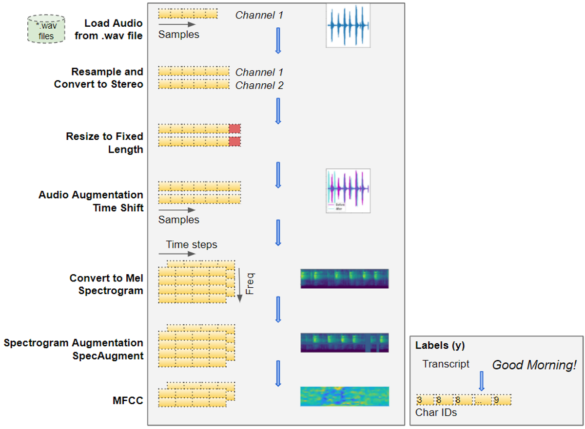Transforming raw audio waves to spectrogram images for input to a deep learning model (Image by Author)

Load Audio Files

• Start with input data that consists of audio files of the spoken speech in an audio format such as “.wav” or “.mp3”.
• Read the audio data from the file and load it into a 2D Numpy array. This array consists of a sequence of numbers, each representing a measurement of the intensity or amplitude of the sound at a particular moment in time. The number of such measurements is determined by the sampling rate. For instance, if the sampling rate was 44.1kHz, the Numpy array will have a single row of 44,100 numbers for 1 second of audio.
• Audio can have one or two channels, known as mono or stereo, in common parlance. With two-channel audio, we would have another similar sequence of amplitude numbers for the second channel. In other words, our Numpy array will be 3D, with a depth of 2.

Convert to uniform dimensions: sample rate, channels, and duration

• We might have a lot of variation in our audio data items. Clips might be sampled at different rates, or have a different number of channels. The clips will most likely have different durations. As explained above this means that the dimensions of each audio item will be different.
• Since our deep learning models expect all our input items to have a similar size, we now perform some data cleaning steps to standardize the dimensions of our audio data. We resample the audio so that every item has the same sampling rate. We convert all items to the same number of channels. All items also have to be converted to the same audio duration. This involves padding the shorter sequences or truncating the longer sequences.
• If the quality of the audio was poor, we might enhance it by applying a noise-removal algorithm to eliminate background noise so that we can focus on the spoken audio.

Data Augmentation of raw audio

• We could apply some data augmentation techniques to add more variety to our input data and help the model learn to generalize to a wider range of inputs. We could Time Shift our audio left or right randomly by a small percentage, or change the Pitch or the Speed of the audio by a small amount.

Mel Spectrograms

• This raw audio is now converted to Mel Spectrograms. A Spectrogram captures the nature of the audio as an image by decomposing it into the set of frequencies that are included in it.

MFCC

• For human speech, in particular, it sometimes helps to take one additional step and convert the Mel Spectrogram into MFCC (Mel Frequency Cepstral Coefficients). MFCCs produce a compressed representation of the Mel Spectrogram by extracting only the most essential frequency coefficients, which correspond to the frequency ranges at which humans speak.

Data Augmentation of Spectrograms

• We can now apply another data augmentation step on the Mel Spectrogram images, using a technique known as SpecAugment. This involves Frequency and Time Masking that randomly masks out either vertical (ie. Time Mask) or horizontal (ie. Frequency Mask) bands of information from the Spectrogram. NB: I’m not sure whether this can also be applied to MFCCs and whether that produces good results.

We have now transformed our original raw audio file into Mel Spectrogram (or MFCC) images after data cleaning and augmentation.

We also need to prepare the target labels from the transcript. This is simply regular text consisting of sentences of words, so we build a vocabulary from each character in the transcript and convert them into character IDs.

This gives us our input features and our target labels. This data is ready to be input into our deep learning model.

Architecture

There are many variations of deep learning architecture for ASR. Two commonly used approaches are:

• A CNN plus RNN-based architecture that uses the CTC Loss algorithm to demarcate each character of the words in the speech. eg. Baidu’s Deep Speech model.
• An RNN-based sequence-to-sequence network that treats each ‘slice’ of the spectrogram as one element in a sequence eg. Google’s Listen Attend Spell (LAS) model.

Let’s pick the first approach above and explore in more detail how that works. At a high level, the model consists of these blocks:

• A regular convolutional network consisting of a few Residual CNN layers that process the input spectrogram images and output feature maps of those images.

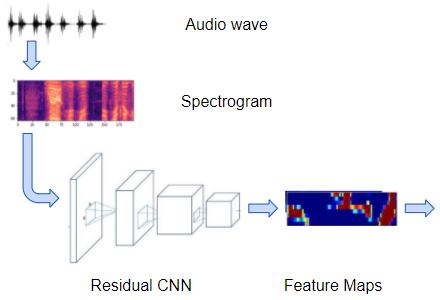Spectrograms are processed by a convolutional network to produce feature maps (Image by Author)

• A regular recurrent network consisting of a few Bidirectional LSTM layers that process the feature maps as a series of distinct timesteps or ‘frames’ that correspond to our desired sequence of output characters. In other words, it takes the feature maps which are a continuous representation of the audio, and converts them into a discrete representation.

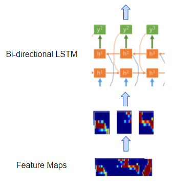Recurrent network processes frames from the feature maps (Image by Author)

• A linear layer with softmax that uses the LSTM outputs to produce character probabilities for each timestep of the output.

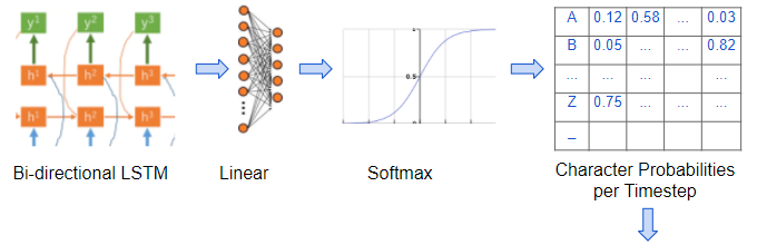Linear layer generates character probabilities for each timestep (Image by Author)

• We also have linear layers that sit between the convolution and recurrent networks and help to reshape the outputs of one network to the inputs of the other.

So our model takes the Spectrogram images and outputs character probabilities for each timestep or ‘frame’ in that Spectrogram.

Align the sequences

If you think about this a little bit, you’ll realize that there is still a major missing piece in our puzzle. Our eventual goal is to map those timesteps or ‘frames’ to individual characters in our target transcript.

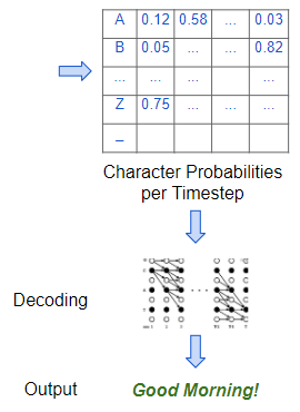The model decodes the character probabilities to produce the final output (Image by Author)

But for a particular spectrogram, how do we know how many frames there should be? How do we know exactly where the boundaries of each frame are? How do we align the audio with each character in the text transcript?

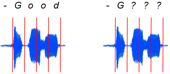On the left is the alignment we need. But how do we get it?? (Image by Author)

The audio and the spectrogram images are not pre-segmented to give us this information.

• In the spoken audio, and therefore in the spectrogram, the sound of each character could be of different durations.
• There could be gaps and pauses between these characters.
• Several characters could be merged together.
• Some characters could be repeated. eg. in the word ‘apple’, how do we know whether that “p” sound in the audio actually corresponds to one or two “p”s in the transcript?

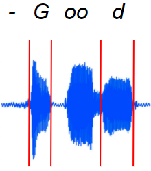In reality, spoken speech is not neatly aligned for us (Image by Author)

This is actually a very challenging problem, and what makes ASR so tough to get right. It is the distinguishing characteristic that differentiates ASR from other audio applications like classification and so on.

The way we tackle this is by using an ingenious algorithm with a fancy-sounding name — it is called Connectionist Temporal Classification, or CTC for short. Since I am not ‘fancy people’ and find it difficult to remember that long name, I will just use the name CTC to refer to it 😃.

CTC Algorithm — Training and Inference

CTC is used to align the input and output sequences when the input is continuous and the output is discrete, and there are no clear element boundaries that can be used to map the input to the elements of the output sequence.

What makes this so special is that it performs this alignment automatically, without requiring you to manually provide that alignment as part of the labeled training data. That would have made it extremely expensive to create the training datasets.

As we discussed above, the feature maps that are output by the convolutional network in our model are sliced into separate frames and input to the recurrent network. Each frame corresponds to some timestep of the original audio wave. However, the number of frames and the duration of each frame are chosen by you as hyperparameters when you design the model. For each frame, the recurrent network followed by the linear classifier then predicts probabilities for each character from the vocabulary.

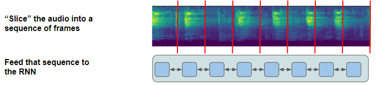The continuous audio is sliced into discrete frames and input to the RNN (Image by Author)

The job of the CTC algorithm is to take these character probabilities and derive the correct sequence of characters.

To help it handle the challenges of alignment and repeated characters that we just discussed, it introduces the concept of a ‘blank’ pseudo-character (denoted by “-”) into the vocabulary. Therefore the character probabilities output by the network also include the probability of the blank character for each frame.

Note that a blank is not the same as a ‘space’. A space is a real character while a blank means the absence of any character, somewhat like a ‘null’ in most programming languages. It is used only to demarcate the boundary between two characters.

CTC works in two modes:

• CTC Loss (during Training): It has a ground truth target transcript and tries to train the network to maximize the probability of outputting that correct transcript.
• CTC Decoding (during Inference): Here we don’t have a target transcript to refer to, and have to predict the most likely sequence of characters.

Let’s explore these a little more to understand what the algorithm does. We’ll start with CTC Decoding as it is a little simpler.

CTC Decoding

Use the character probabilities to pick the most likely character for each frame, including blanks. eg. “-G-o-ood”

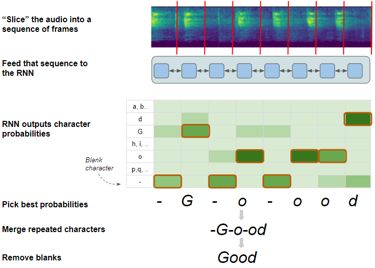CTC Decode algorithm (Image by Author)

• Merge any characters that are repeated, and not separated by a blank. For instance, we can merge the “oo” into a single “o”, but we cannot merge the “o-oo”. This is how the CTC is able to distinguish that there are two separate “o”s and produce words spelled with repeated characters. eg. “-G-o-od”
• Finally, since the blanks have served their purpose, it removes all blank characters. eg. “Good”.

CTC Loss

The Loss is computed as the probability of the network predicting the correct sequence. To do this, the algorithm lists out all possible sequences the network can predict, and from that it selects the subset that match the target transcript.

To identify that subset from the full set of possible sequences, the algorithm narrows down the possibilities as follows:

• Keep only the probabilities for characters that occur in the target transcript and discard the rest. eg. It keeps probabilities only for “G”, “o”, “d”, and “-”.
• Using the filtered subset of characters, for each frame, select only those characters which occur in the same order as the target transcript. eg. Although “G” and “o” are both valid characters, an order of “Go” is a valid sequence whereas “oG” is an invalid sequence.

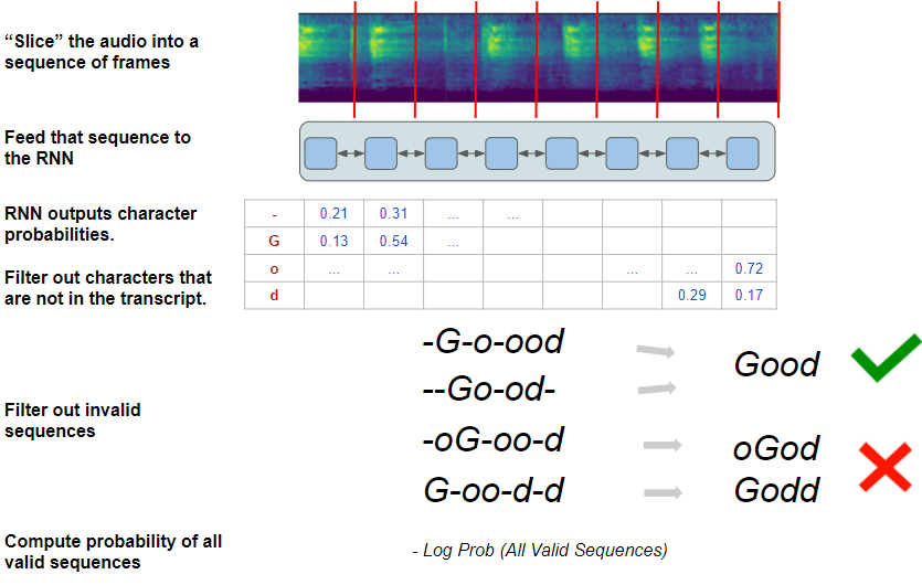CTC Loss algorithm (Image by Author)

With these constraints in place, the algorithm now has a set of valid character sequences, all of which will produce the correct target transcript. eg. Using the same steps that were used during Inference, “-G-o-ood” and “_ — Go-od-_” will both result in a final output of “Good”.

It then uses the individual character probabilities for each frame, to compute the overall probability of generating all of those valid sequences. The goal of the network is to learn how to maximize that probability and therefore reduce the probability of generating any invalid sequence.

Strictly speaking, since a neural network minimizes loss, the CTC Loss is computed as the negative log probability of all valid sequences. As the network minimizes that loss via back-propagation during training, it adjusts all of its weights to produce the correct sequence.

To actually do this, however, is much more complicated than what I’ve described here. The challenge is that there is a huge number of possible combinations of characters to produce a sequence. With our simple example alone, we can have 4 characters per frame. With 8 frames that gives us 4 ** 8 combinations (= 65536). For any realistic transcript with more characters and more frames, this number increases exponentially. That makes it computationally impractical to simply exhaustively list out the valid combinations and compute their probability.

Solving this efficiently is what makes CTC so innovative. It is a fascinating algorithm and it is well worth understanding the nuances of how it achieves this. That merits a complete article by itself which I plan to write shortly. But for now, we have focused on building intuition about what CTC does, rather than going into how it works.

Metrics — Word Error Rate (WER)

After training our network, we must evaluate how well it performs. A commonly used metric for Speech-to-Text problems is the Word Error Rate (and Character Error Rate). It compares the predicted output and the target transcript, word by word (or character by character) to figure out the number of differences between them.

A difference could be a word that is present in the transcript but missing from the prediction (counted as a Deletion), a word that is not in the transcript but has been added into the prediction (an Insertion), or a word that is altered between the prediction and the transcript (a Substitution).

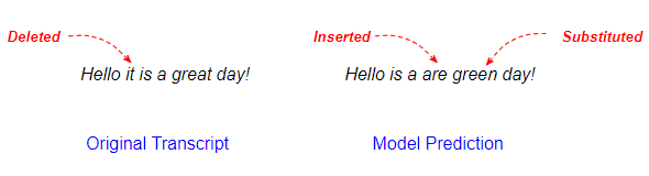Count the Insertions, Deletions, and Substitutions between the Transcript and the Prediction (Image by Author)

The metric formula is fairly straightforward. It is the percent of differences relative to the total number of words.

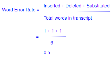Word Error Rate computation (Image by Author)

Language Model

So far, our algorithm has treated the spoken audio as merely corresponding to a sequence of characters from some language. But when put together into words and sentences will those characters actually make sense and have meaning?

A common application in NLP is to build a Language Model. It captures how words are typically used in a language to construct sentences, paragraphs, and documents. It could be a general-purpose model about a language such as English or Korean, or it could be a model that is specific to a particular domain such as medical or legal.

Once you have a Language Model, it can become the foundation for other applications. For instance, it could be used to predict the next word in a sentence, to discern the sentiment of some text (eg. is this a positive book review), to answer questions via a chatbot, and so on.

So, of course, it can also be used to optionally enhance the quality of our ASR outputs by guiding the model to generate predictions that are more likely as per the Language Model.

Beam Search

While describing the CTC Decoder during Inference, we implicitly assumed that it always picks a single character with the highest probability at each timestep. This is known as Greedy Search.

However, we know that we can get better results using an alternative method called Beam Search.

Although Beam Search is often used with NLP problems in general, it is not specific to ASR, so I’m mentioning it here just for completeness. If you’d like to know more, please take a look at my article that describes Beam Search in full detail.

Conclusion

Hopefully, this now gives you a sense of the building blocks and techniques that are used to solve ASR problems.

In the older pre-deep-learning days, tackling such problems via classical approaches required an understanding of concepts like phonemes and a lot of domain-specific data preparation and algorithms.

However, as we’ve just seen with deep learning, we required hardly any feature engineering involving knowledge of audio and speech. And yet, it is able to produce excellent results that continue to surprise us!

And finally, if you liked this article, you might also enjoy my other series on Transformers as well as Reinforcement Learning.

Transformers Explained Visually: Overview of functionality

Reinforcement Learning Made Simple (Part 1): Intro to Basic Concepts and Terminology

Let’s keep learning!