
This is the second article in my series on Transformers. In the first article, we learned about the functionality of Transformers, how they are used, their high-level architecture, and their advantages.
In this article, we can now look under the hood and study exactly how they work in detail. We’ll see how data flows through the system with their actual matrix representations and shapes and understand the computations performed at each stage.
Here’s a quick summary of the previous and following articles in the series. My goal throughout will be to understand not just how something works but why it works that way.
- Overview of functionality (How Transformers are used, and why they are better than RNNs. Components of the architecture, and behavior during Training and Inference)
- How it works — this article (Internal operation end-to-end. How data flows and what computations are performed, including matrix representations)
- Multi-head Attention (Inner workings of the Attention module throughout the Transformer)
- Why Attention Boosts Performance (Not just what Attention does but why it works so well. How does Attention capture the relationships between words in a sentence)
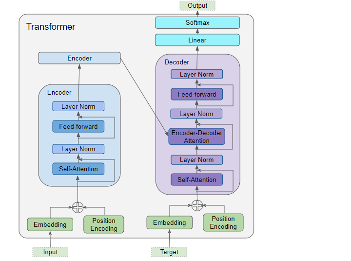
Architecture Overview
As we saw in Part 1, the main components of the architecture are:
 (Image by Author)
Data inputs for both the Encoder and Decoder, which contains:
- Embedding layer
- Position Encoding layer
The Encoder stack contains a number of Encoders. Each Encoder contains:
- Multi-Head Attention layer
- Feed-forward layer
The Decoder stack contains a number of Decoders. Each Decoder contains:
- Two Multi-Head Attention layers
- Feed-forward layer
Output (top right) — generates the final output, and contains:
- Linear layer
- Softmax layer.
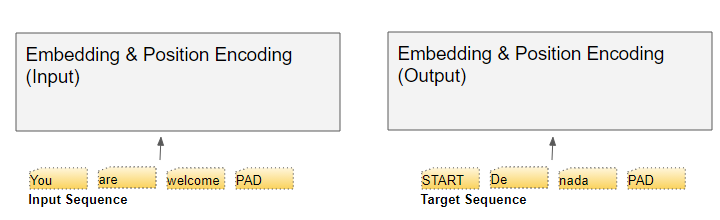
To understand what each component does, let’s walk through the working of the Transformer while we are training it to solve a translation problem. We’ll use one sample of our training data which consists of an input sequence (‘You are welcome’ in English) and a target sequence (‘De nada’ in Spanish).
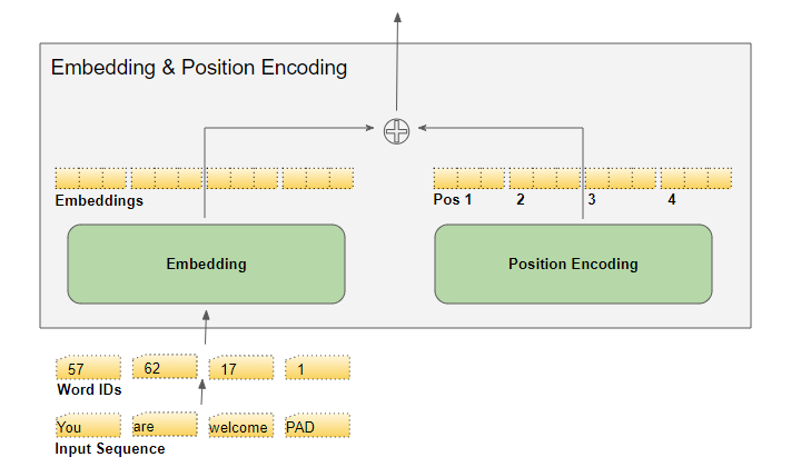
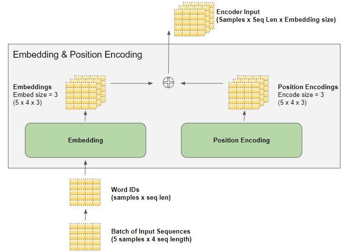
Embedding and Position Encoding
Like any NLP model, the Transformer needs two things about each word — the meaning of the word and its position in the sequence.
- The Embedding layer encodes the meaning of the word.
- The Position Encoding layer represents the position of the word.
The Transformer combines these two encodings by adding them.
Embedding
The Transformer has two Embedding layers. The input sequence is fed to the first Embedding layer, known as the Input Embedding.
 (Image by Author)
The target sequence is fed to the second Embedding layer after shifting the targets right by one position and inserting a Start token in the first position. Note that, during Inference, we have no target sequence and we feed the output sequence to this second layer in a loop, as we learned in Part 1. That is why it is called the Output Embedding.
The text sequence is mapped to numeric word IDs using our vocabulary. The embedding layer then maps each input word into an embedding vector, which is a richer representation of the meaning of that word.
 (Image by Author)
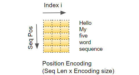
Position Encoding
Since an RNN implements a loop where each word is input sequentially, it implicitly knows the position of each word.
However, Transformers don’t use RNNs and all words in a sequence are input in parallel. This is its major advantage over the RNN architecture, but it means that the position information is lost, and has to be added back in separately.
Just like the two Embedding layers, there are two Position Encoding layers. The Position Encoding is computed independently of the input sequence. These are fixed values that depend only on the max length of the sequence. For instance,
- the first item is a constant code that indicates the first position
- the second item is a constant code that indicates the second position,
- and so on.
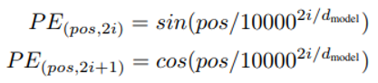
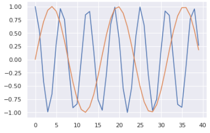
These constants are computed using the formula below, where
 (Image by Author)
- pos is the position of the word in the sequence
- d_model is the length of the encoding vector (same as the embedding vector) and
- i is the index value into this vector.
 (Image by Author)
In other words, it interleaves a sine curve and a cos curve, with sine values for all even indexes and cos values for all odd indexes. As an example, if we encode a sequence of 40 words, we can see below the encoding values for a few (word position, encoding_index) combinations.
 (Image by Author)
The blue curve shows the encoding of the 0th index for all 40 word-positions and the orange curve shows the encoding of the 1st index for all 40 word-positions. There will be similar curves for the remaining index values.
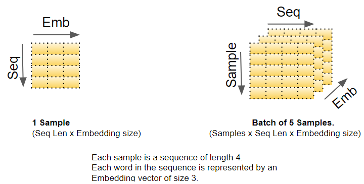
Matrix Dimensions
As we know, deep learning models process a batch of training samples at a time. The Embedding and Position Encoding layers operate on matrices representing a batch of sequence samples. The Embedding takes a (samples, sequence length) shaped matrix of word IDs. It encodes each word ID into a word vector whose length is the embedding size, resulting in a (samples, sequence length, embedding size) shaped output matrix. The Position Encoding uses an encoding size that is equal to the embedding size. So it produces a similarly shaped matrix that can be added to the embedding matrix.
 (Image by Author)
The (samples, sequence length, embedding size) shape produced by the Embedding and Position Encoding layers is preserved all through the Transformer, as the data flows through the Encoder and Decoder Stacks until it is reshaped by the final Output layers.
This gives a sense of the 3D matrix dimensions in the Transformer. However, to simplify the visualization, from here on we will drop the first dimension (for the samples) and use the 2D representation for a single sample.
 (Image by Author)
The Input Embedding sends its outputs into the Encoder. Similarly, the Output Embedding feeds into the Decoder.
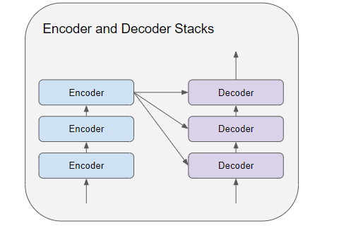
Encoder
The Encoder and Decoder Stacks consists of several (usually six) Encoders and Decoders respectively, connected sequentially.
 (Image by Author)
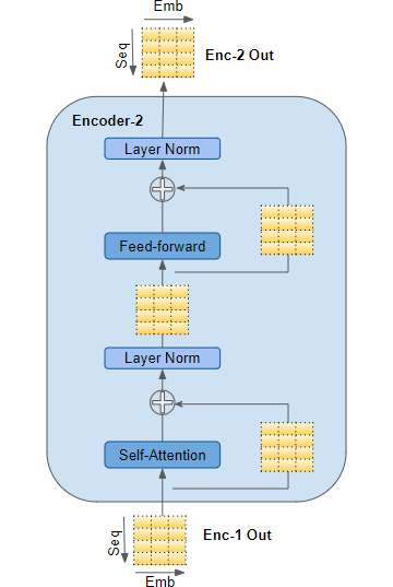
The first Encoder in the stack receives its input from the Embedding and Position Encoding. The other Encoders in the stack receive their input from the previous Encoder.
The Encoder passes its input into a Multi-head Self-attention layer. The Self-attention output is passed into a Feed-forward layer, which then sends its output upwards to the next Encoder.
 (Image by Author)
Both the Self-attention and Feed-forward sub-layers, have a residual skip-connection around them, followed by a Layer-Normalization.
The output of the last Encoder is fed into each Decoder in the Decoder Stack as explained below.
Decoder
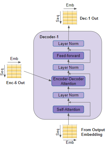
The Decoder’s structure is very similar to the Encoder’s but with a couple of differences.
Like the Encoder, the first Decoder in the stack receives its input from the Output Embedding and Position Encoding. The other Decoders in the stack receive their input from the previous Decoder.
The Decoder passes its input into a Multi-head Self-attention layer. This operates in a slightly different way than the one in the Encoder. It is only allowed to attend to earlier positions in the sequence. This is done by masking future positions, which we’ll talk about shortly.
 (Image by Author)
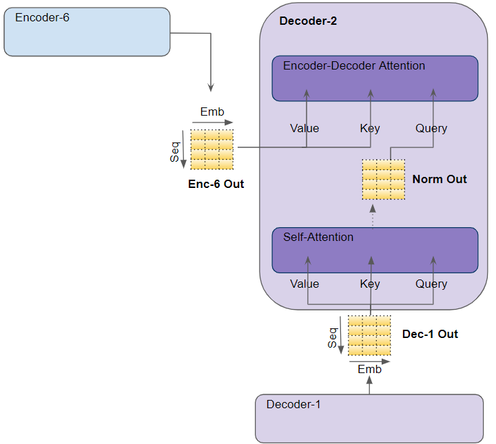
Unlike the Encoder, the Decoder has a second Multi-head attention layer, known as the Encoder-Decoder attention layer. The Encoder-Decoder attention layer works like Self-attention, except that it combines two sources of inputs — the Self-attention layer below it as well as the output of the Encoder stack.
The Self-attention output is passed into a Feed-forward layer, which then sends its output upwards to the next Decoder.
Each of these sub-layers, Self-attention, Encoder-Decoder attention, and Feed-forward, have a residual skip-connection around them, followed by a Layer-Normalization.
Attention
In Part 1, we talked about why Attention is so important while processing sequences. In the Transformer, Attention is used in three places:
- Self-attention in the Encoder — the input sequence pays attention to itself
- Self-attention in the Decoder — the target sequence pays attention to itself
- Encoder-Decoder-attention in the Decoder — the target sequence pays attention to the input sequence
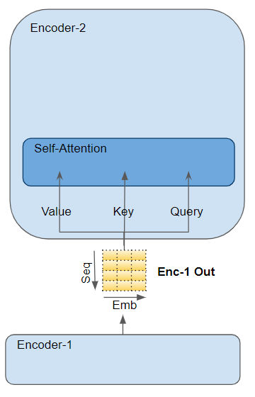
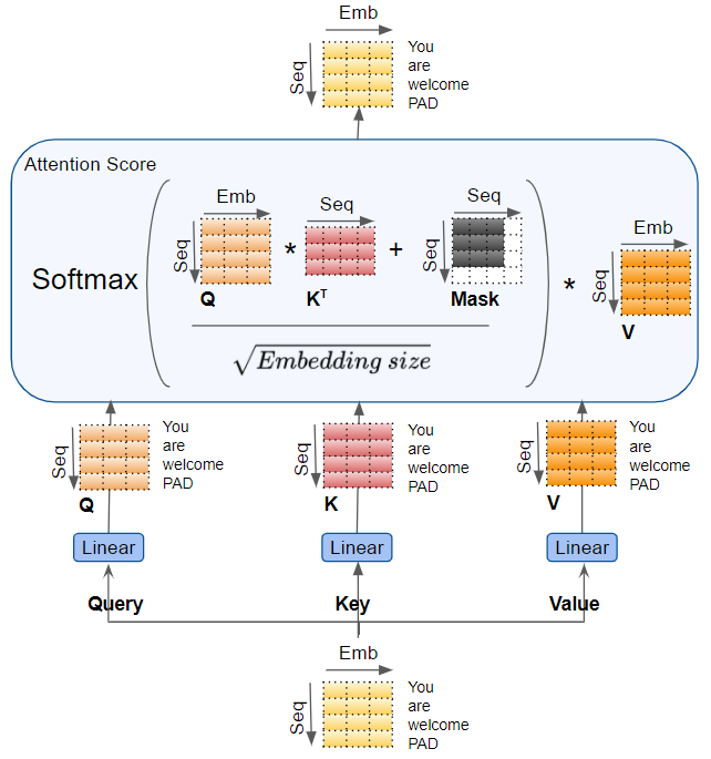
The Attention layer takes its input in the form of three parameters, known as the Query, Key, and Value.
- In the Encoder’s Self-attention, the Encoder’s input is passed to all three parameters, Query, Key, and Value.
 (Image by Author)
- In the Decoder’s Self-attention, the Decoder’s input is passed to all three parameters, Query, Key, and Value.
- In the Decoder’s Encoder-Decoder attention, the output of the final Encoder in the stack is passed to the Value and Key parameters. The output of the Self-attention (and Layer Norm) module below it is passed to the Query parameter.
 (Image by Author)
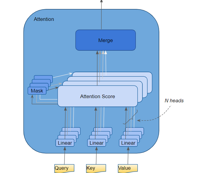
Multi-head Attention
The Transformer calls each Attention processor an Attention Head and repeats it several times in parallel. This is known as Multi-head attention. It gives its Attention greater power of discrimination, by combining several similar Attention calculations.
 (Image by Author)
The Query, Key, and Value are each passed through separate Linear layers, each with their own weights, producing three results called Q, K, and V respectively. These are then combined together using the Attention formula as shown below, to produce the Attention Score.
 (Image by Author)
The important thing to realize here is that the Q, K, and V values carry an encoded representation of each word in the sequence. The Attention calculations then combine each word with every other word in the sequence, so that the Attention Score encodes a score for each word in the sequence.
When discussing the Decoder a little while back, we briefly mentioned masking. The Mask is also shown in the Attention diagrams above. Let’s see how it works.
Attention Masks
While computing the Attention Score, the Attention module implements a masking step. Masking serves two purposes:
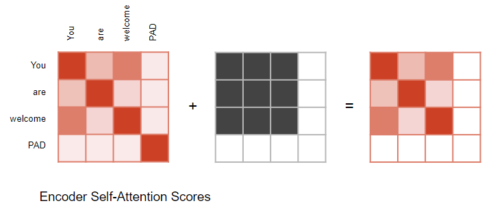
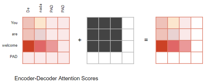
In the Encoder Self-attention and in the Encoder-Decoder-attention: masking serves to zero attention outputs where there is padding in the input sentences, to ensure that padding doesn’t contribute to the self-attention. (Note: since input sequences could be of different lengths they are extended with padding tokens like in most NLP applications so that fixed-length vectors can be input to the Transformer.)
 (Image by Author)
Similarly for the Encoder-Decoder attention.
 (Image by Author)
In the Decoder Self-attention: masking serves to prevent the decoder from ‘peeking’ ahead at the rest of the target sentence when predicting the next word.
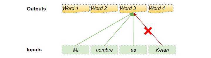
The Decoder processes words in the source sequence and uses them to predict the words in the destination sequence. During training, this is done via Teacher Forcing, where the complete target sequence is fed as Decoder inputs. Therefore, while predicting a word at a certain position, the Decoder has available to it the target words preceding that word as well as the target words following that word. This allows the Decoder to ‘cheat’ by using target words from future ‘time steps’.
For instance, when predicting ‘Word 3’, the Decoder should refer only to the first 3 input words from the target but not the fourth word ‘Ketan’.
 (Image by Author)
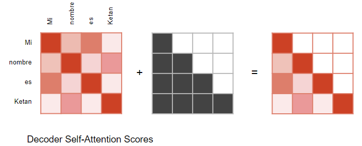
Therefore, the Decoder masks out input words that appear later in the sequence.
 (Image by Author)
When calculating the Attention Score (refer to the picture earlier showing the calculations) masking is applied to the numerator just before the Softmax. The masked out elements (white squares) are set to negative infinity, so that Softmax turns those values to zero.
Generate Output
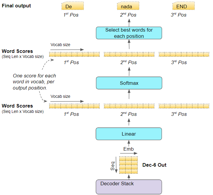
The last Decoder in the stack passes its output to the Output component which converts it into the final output sentence.
The Linear layer projects the Decoder vector into Word Scores, with a score value for each unique word in the target vocabulary, at each position in the sentence. For instance, if our final output sentence has 7 words and the target Spanish vocabulary has 10000 unique words, we generate 10000 score values for each of those 7 words. The score values indicate the likelihood of occurrence for each word in the vocabulary in that position of the sentence.
The Softmax layer then turns those scores into probabilities (which add up to 1.0). In each position, we find the index for the word with the highest probability, and then map that index to the corresponding word in the vocabulary. Those words then form the output sequence of the Transformer.
 (Image by Author)
Training and Loss Function
During training, we use a loss function such as cross-entropy loss to compare the generated output probability distribution to the target sequence. The probability distribution gives the probability of each word occurring in that position.
 (Image by Author)
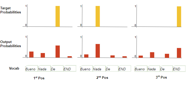
Let’s assume our target vocabulary contains just four words. Our goal is to produce a probability distribution that matches our expected target sequence “De nada END”.
This means that the probability distribution for the first word-position should have a probability of 1 for “De” with probabilities for all other words in the vocabulary being 0. Similarly, “nada” and “END” should have a probability of 1 for the second and third word-positions respectively.
As usual, the loss is used to compute gradients to train the Transformer via backpropagation.
Conclusion
Hopefully, this gives you a feel for what goes on inside the Transformer during Training. As we discussed in the previous article, it runs in a loop during Inference but most of the processing remains the same.
The Multi-head Attention module is what gives the Transformer its power. In the next article, we will continue our journey and go one step deeper to really understand the details of how Attention is computed.
And finally, if you are interested in NLP, you might also enjoy my article on Beam Search, and my other series on Audio Deep Learning and Reinforcement Learning.
Reinforcement Learning Made Simple (Part 1): Intro to Basic Concepts and Terminology
Let’s keep learning!