
This is the third article in my series on Transformers. We are covering its functionality in a top-down manner. In the previous articles, we learned what a Transformer is, its architecture, and how it works.
In this article, we will go a step further and dive deeper into Multi-head Attention, which is the brains of the Transformer.
Here’s a quick summary of the previous and following articles in the series. My goal throughout will be to understand not just how something works but why it works that way.
- Overview of functionality (How Transformers are used, and why they are better than RNNs. Components of the architecture, and behavior during Training and Inference)
- How it works (Internal operation end-to-end. How data flows and what computations are performed, including matrix representations)
- Multi-head Attention — this article (Inner workings of the Attention module throughout the Transformer)
- Why Attention Boosts Performance (Not just what Attention does but why it works so well. How does Attention capture the relationships between words in a sentence)
If you haven’t read the previous articles, it might be a good idea to read them first, as this article builds on many of the concepts that we covered there.
How Attention is used in the Transformer
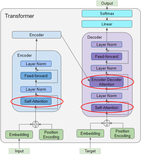
As we discussed in Part 2, Attention is used in the Transformer in three places:
- Self-attention in the Encoder — the input sequence pays attention to itself
- Self-attention in the Decoder — the target sequence pays attention to itself
- Encoder-Decoder-attention in the Decoder — the target sequence pays attention to the input sequence
 (Image by Author)
Attention Input Parameters — Query, Key, and Value
The Attention layer takes its input in the form of three parameters, known as the Query, Key, and Value.
All three parameters are similar in structure, with each word in the sequence represented by a vector.
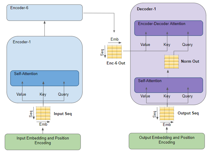
Encoder Self-Attention
The input sequence is fed to the Input Embedding and Position Encoding, which produces an encoded representation for each word in the input sequence that captures the meaning and position of each word. This is fed to all three parameters, Query, Key, and Value in the Self-Attention in the first Encoder which then also produces an encoded representation for each word in the input sequence, that now incorporates the attention scores for each word as well. As this passes through all the Encoders in the stack, each Self-Attention module also adds its own attention scores into each word’s representation.
 (Image by Author)
Decoder Self-Attention
Coming to the Decoder stack, the target sequence is fed to the Output Embedding and Position Encoding, which produces an encoded representation for each word in the target sequence that captures the meaning and position of each word. This is fed to all three parameters, Query, Key, and Value in the Self-Attention in the first Decoder which then also produces an encoded representation for each word in the target sequence, which now incorporates the attention scores for each word as well.
After passing through the Layer Norm, this is fed to the Query parameter in the Encoder-Decoder Attention in the first Decoder
Encoder-Decoder Attention
Along with that, the output of the final Encoder in the stack is passed to the Value and Key parameters in the Encoder-Decoder Attention.
The Encoder-Decoder Attention is therefore getting a representation of both the target sequence (from the Decoder Self-Attention) and a representation of the input sequence (from the Encoder stack). It, therefore, produces a representation with the attention scores for each target sequence word that captures the influence of the attention scores from the input sequence as well.
As this passes through all the Decoders in the stack, each Self-Attention and each Encoder-Decoder Attention also add their own attention scores into each word’s representation.
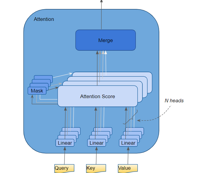
Multiple Attention Heads
In the Transformer, the Attention module repeats its computations multiple times in parallel. Each of these is called an Attention Head. The Attention module splits its Query, Key, and Value parameters N-ways and passes each split independently through a separate Head. All of these similar Attention calculations are then combined together to produce a final Attention score. This is called Multi-head attention and gives the Transformer greater power to encode multiple relationships and nuances for each word.
 (Image by Author)
To understand exactly how the data is processed internally, let’s walk through the working of the Attention module while we are training the Transformer to solve a translation problem. We’ll use one sample of our training data which consists of an input sequence (‘You are welcome’ in English) and a target sequence (‘De nada’ in Spanish).
Attention Hyperparameters
There are three hyperparameters that determine the data dimensions:
- Embedding Size — width of the embedding vector (we use a width of 6 in our example). This dimension is carried forward throughout the Transformer model and hence is sometimes referred to by other names like ‘model size’ etc.
- Query Size (equal to Key and Value size)— the size of the weights used by three Linear layers to produce the Query, Key, and Value matrices respectively (we use a Query size of 3 in our example)
- Number of Attention heads (we use 2 heads in our example)
In addition, we also have the Batch size, giving us one dimension for the number of samples.
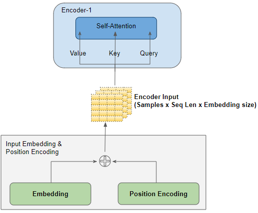
Input Layers
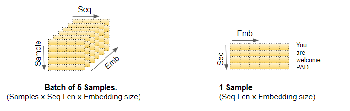
The Input Embedding and Position Encoding layers produce a matrix of shape (Number of Samples, Sequence Length, Embedding Size) which is fed to the Query, Key, and Value of the first Encoder in the stack.
 (Image by Author)
To make it simple to visualize, we will drop the Batch dimension in our pictures and focus on the remaining dimensions.
 (Image by Author)
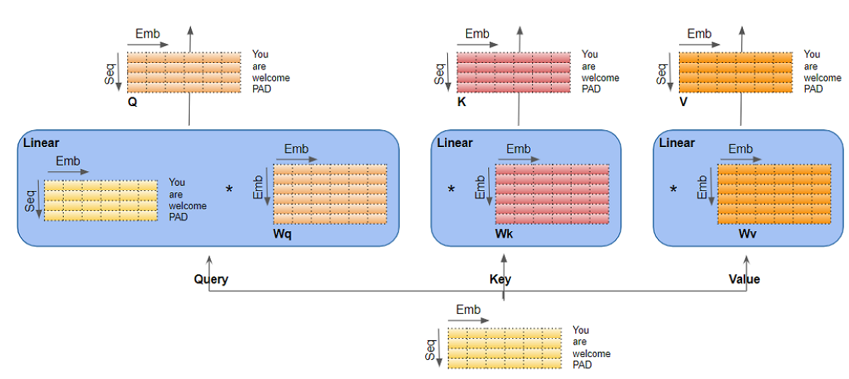
Linear Layers
There are three separate Linear layers for the Query, Key, and Value. Each Linear layer has its own weights. The input is passed through these Linear layers to produce the Q, K, and V matrices.
 (Image by Author)
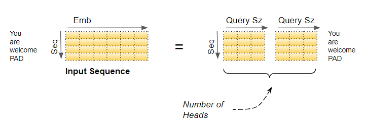
Splitting data across Attention heads
Now the data gets split across the multiple Attention heads so that each can process it independently.
However, the important thing to understand is that this is a logical split only. The Query, Key, and Value are not physically split into separate matrices, one for each Attention head. A single data matrix is used for the Query, Key, and Value, respectively, with logically separate sections of the matrix for each Attention head. Similarly, there are not separate Linear layers, one for each Attention head. All the Attention heads share the same Linear layer but simply operate on their ‘own’ logical section of the data matrix.
Linear layer weights are logically partitioned per head
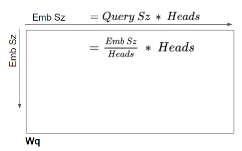
This logical split is done by partitioning the input data as well as the Linear layer weights uniformly across the Attention heads. We can achieve this by choosing the Query Size as below:
Query Size = Embedding Size / Number of heads
 (Image by Author)
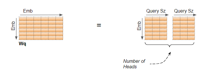
In our example, that is why the Query Size = 6/2 = 3. Even though the layer weight (and input data) is a single matrix we can think of it as ‘stacking together’ the separate layer weights for each head.
 (Image by Author)
The computations for all Heads can be therefore be achieved via a single matrix operation rather than requiring N separate operations. This makes the computations more efficient and keeps the model simple because fewer Linear layers are required, while still achieving the power of the independent Attention heads.
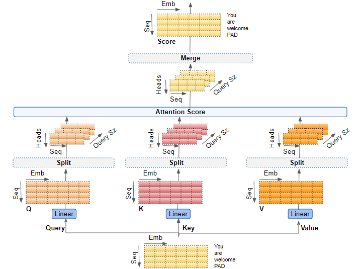
Reshaping the Q, K, and V matrices
The Q, K, and V matrices output by the Linear layers are reshaped to include an explicit Head dimension. Now each ‘slice’ corresponds to a matrix per head.
This matrix is reshaped again by swapping the Head and Sequence dimensions. Although the Batch dimension is not drawn, the dimensions of Q are now (Batch, Head, Sequence, Query size).
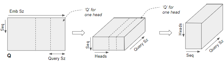 The Q matrix is reshaped to include a Head dimension and then reshaped again by swapping the Head and Sequencd dimensions. (Image by Author)
In the picture below, we can see the complete process of splitting our example Q matrix, after coming out of the Linear layer.
The final stage is for visualization only — although the Q matrix is a single matrix, we can think of it as a logically separate Q matrix per head.
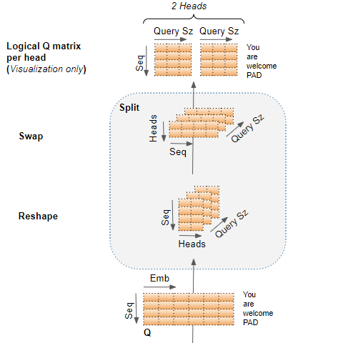 Q matrix split across the Attention Heads (Image by Author)
We are ready to compute the Attention Score.
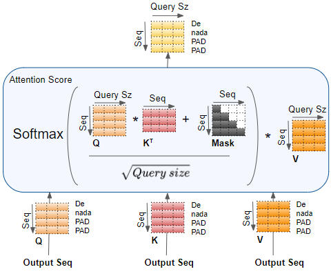
Compute the Attention Score for each head
We now have the 3 matrices, Q, K, and V, split across the heads. These are used to compute the Attention Score.
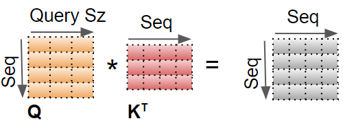
We will show the computations for a single head using just the last two dimensions (Sequence and Query size) and skip the first two dimensions (Batch and Head). Essentially, we can imagine that the computations we’re looking at are getting ‘repeated’ for each head and for each sample in the batch (although, obviously, they are happening as a single matrix operation, and not as a loop).
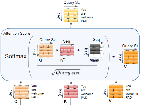
The first step is to do a matrix multiplication between Q and K.
 (Image by Author)
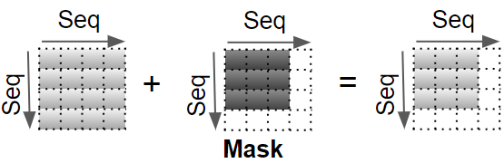
A Mask value is now added to the result. In the Encoder Self-attention, the mask is used to mask out the Padding values so that they don’t participate in the Attention Score.
Different masks are applied in the Decoder Self-attention and in the Decoder Encoder-Attention which we’ll come to a little later in the flow.
 (Image by Author)
The result is now scaled by dividing by the square root of the Query size, and then a Softmax is applied to it.
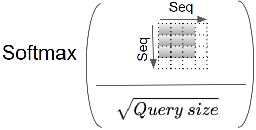 (Image by Author)
Another matrix multiplication is performed between the output of the Softmax and the V matrix.
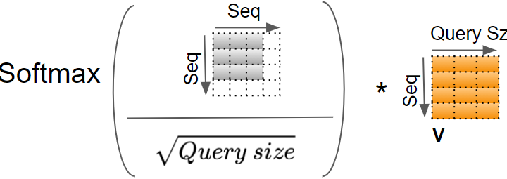 (Image by Author)
The complete Attention Score calculation in the Encoder Self-attention is as below:
 (Image by Author)
Merge each Head’s Attention Scores together
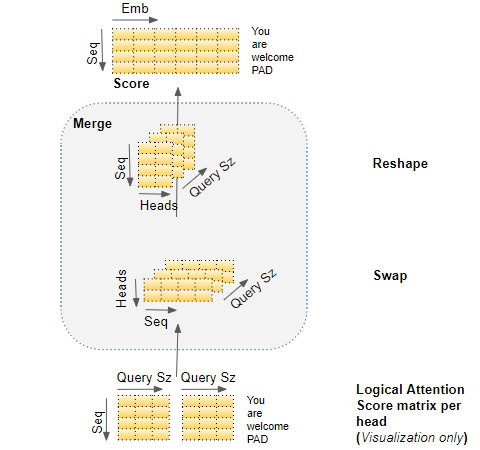
We now have separate Attention Scores for each head, which need to be combined together into a single score. This Merge operation is essentially the reverse of the Split operation.
It is done by simply reshaping the result matrix to eliminate the Head dimension. The steps are:
- Reshape the Attention Score matrix by swapping the Head and Sequence dimensions. In other words, the matrix shape goes from (Batch, Head, Sequence, Query size) to (Batch, Sequence, Head, Query size).
- Collapse the Head dimension by reshaping to (Batch, Sequence, Head * Query size). This effectively concatenates the Attention Score vectors for each head into a single merged Attention Score.
Since Embedding size =Head * Query size, the merged Score is (Batch, Sequence, Embedding size). In the picture below, we can see the complete process of merging for the example Score matrix.
 (Image by Author)
End-to-end Multi-head Attention
Putting it all together, this is the end-to-end flow of the Multi-head Attention.
 (Image by Author)
Multi-head split captures richer interpretations
An Embedding vector captures the meaning of a word. In the case of Multi-head Attention, as we have seen, the Embedding vectors for the input (and target) sequence gets logically split across multiple heads. What is the significance of this?
 (Image by Author)
This means that separate sections of the Embedding can learn different aspects of the meanings of each word, as it relates to other words in the sequence. This allows the Transformer to capture richer interpretations of the sequence.
This may not be a realistic example, but it might help to build intuition. For instance, one section might capture the ‘gender-ness’ (male, female, neuter) of a noun while another might capture the ‘cardinality’ (singular vs plural) of a noun. This might be important during translation because, in many languages, the verb that needs to be used depends on these factors.
Decoder Self-Attention and Masking
The Decoder Self-Attention works just like the Encoder Self-Attention, except that it operates on each word of the target sequence.
 (Image by Author)
Similarly, the Masking masks out the Padding words in the target sequence.
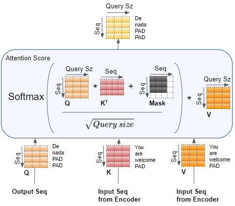
Decoder Encoder-Decoder Attention and Masking
The Encoder-Decoder Attention takes its input from two sources. Therefore, unlike the Encoder Self-Attention, which computes the interaction between each input word with other input words, and Decoder Self-Attention which computes the interaction between each target word with other target words, the Encoder-Decoder Attention computes the interaction between each target word with each input word.
 (Image by Author)
Therefore each cell in the resulting Attention Score corresponds to the interaction between one Q (ie. target sequence word) with all other K (ie. input sequence) words and all V (ie. input sequence) words.
Similarly, the Masking masks out the later words in the target output, as was explained in detail in the second article of the series.
Conclusion
Hopefully, this gives you a good sense of what the Attention modules in the Transformer do. When put together with the end-to-end flow of the Transformer as a whole that we went over in the second article, we have now covered the detailed operation of the entire Transformer architecture.
We now understand exactly what the Transformer does. But we haven’t fully answered the question of why the Transformer’s Attention performs the calculations that it does. Why does it use the notions of Query, Key, and Value, and why does it perform the matrix multiplications that we just saw?
We have a vague intuitive idea that it ‘captures the relationship between each word with each other word’, but what exactly does that mean? How exactly does that give the Transformer’s Attention the capability to understand the nuances of each word in the sequence?
That is an interesting question and is the subject of the final article of this series. Once we learn that, we will truly understand the elegance of the Transformer architecture.
And finally, if you are interested in NLP, you might also enjoy my article on Beam Search, and my other series on Audio Deep Learning and Reinforcement Learning.
Reinforcement Learning Made Simple (Part 1): Intro to Basic Concepts and Terminology
Let’s keep learning!