
This is the sixth article in my series on Reinforcement Learning (RL). We now have a good understanding of the concepts that form the building blocks of an RL problem, and the techniques used to solve them. We have also taken a detailed look at two Value-based algorithms — Q-Learning algorithm and Deep Q Networks (DQN), which was our first step into Deep Reinforcement Learning.
In this article, we will continue our Deep Reinforcement Learning journey and learn about our first Policy-based algorithm using the technique of Policy Gradients. We’ll go through the REINFORCE algorithm step-by-step, so we can see how it contrasts with the DQN approach.
Here’s a quick summary of the previous and following articles in the series. My goal throughout will be to understand not just how something works but why it works that way.
- Intro to Basic Concepts and Terminology (What is an RL problem, and how to apply an RL problem-solving framework to it using techniques from Markov Decision Processes and concepts such as Return, Value, and Policy)
- Solution Approaches (Overview of popular RL solutions, and categorizing them based on the relationship between these solutions. Important takeaways from the Bellman equation, which is the foundation for all RL algorithms.)
- Model-free algorithms (Similarities and differences of Value-based and Policy-based solutions using an iterative algorithm to incrementally improve predictions. Exploitation, Exploration, and ε-greedy policies.)
- Q-Learning (In-depth analysis of this algorithm, which is the basis for subsequent deep-learning approaches. Develop intuition about why this algorithm converges to the optimal values.)
- Deep Q Networks (Our first deep-learning algorithm. A step-by-step walkthrough of exactly how it works, and why those architectural choices were made.)
- Policy Gradient — this article (Our first policy-based deep-learning algorithm.)
- Actor-Critic (Sophisticated deep-learning algorithm which combines the best of Deep Q Networks and Policy Gradients.)
If you haven’t read the earlier articles, it would be a good idea to read them first, as this article builds on many of the concepts that we discussed there.
Policy Gradients
With Deep Q Networks, we obtain the Optimal Policy indirectly. The network learns to output the Optimal Q values for a given state. Those Q values are then used to derive the Optimal Policy.
Because of this, it needs to make use of an implicit policy so that it can train itself eg. it uses an ε-greedy policy.
On the other hand, we could build a neural network that directly learns the Optimal Policy. Rather than learning a function that takes a state as input and outputs Q values for all actions, it instead learns a function that outputs the best action that can be taken from that state.
More precisely, rather than a single best action, it outputs a probability distribution of the actions that can be taken from that state. An action can then be chosen by sampling from the probability distribution.
 (Image by Author)
That is exactly what the Optimal Policy is.
Architecture Components
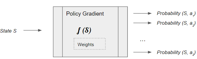
The Policy Network is a fairly standard neural network architecture, which gets trained to predict the Optimal Policy. As with a DQN, it could be as simple as a linear network with a couple of hidden layers if your state can be represented via a set of numeric variables. Or if your state data is represented as images or text, you might use a regular CNN or RNN architecture.
The Policy network takes the current state and predicts a probability distribution of actions to be taken from that state.
 (Image by Author)
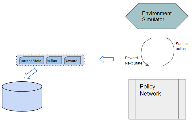
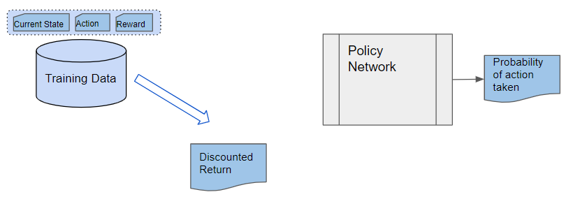
Training data is gathered from actual experience while interacting with the environment and storing the observed results. An episode of experience is stored. Each sample consists of a (state, action, reward) tuple.
High-level Workflow
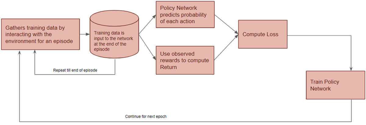
The high-level workflow is that the Policy Gradient gets trained over many epochs. There are two phases per epoch. In the first phase, it gathers training data from the environment for an episode. In the second phase, it uses the training data to train the Policy Network.
 (Image by Author)
Now let’s zoom in on this first phase.
 (Image by Author)
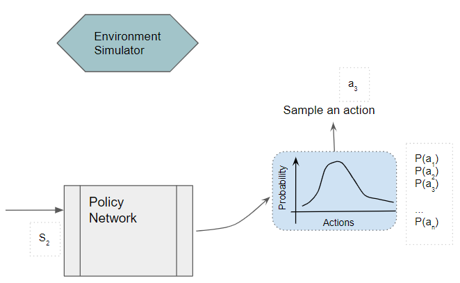
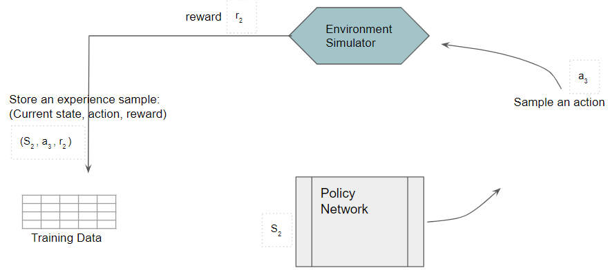
The Policy Network acts as the agent and interacts with the environment for an episode. From the current state, the Policy Network predicts a probability distribution of actions. It then samples an action from this distribution, executes it with the environment, and gets back a reward and the next state. It saves each observation as a sample of training data.
The Policy Network remains fixed and does not improve during this phase.
 (Image by Author)
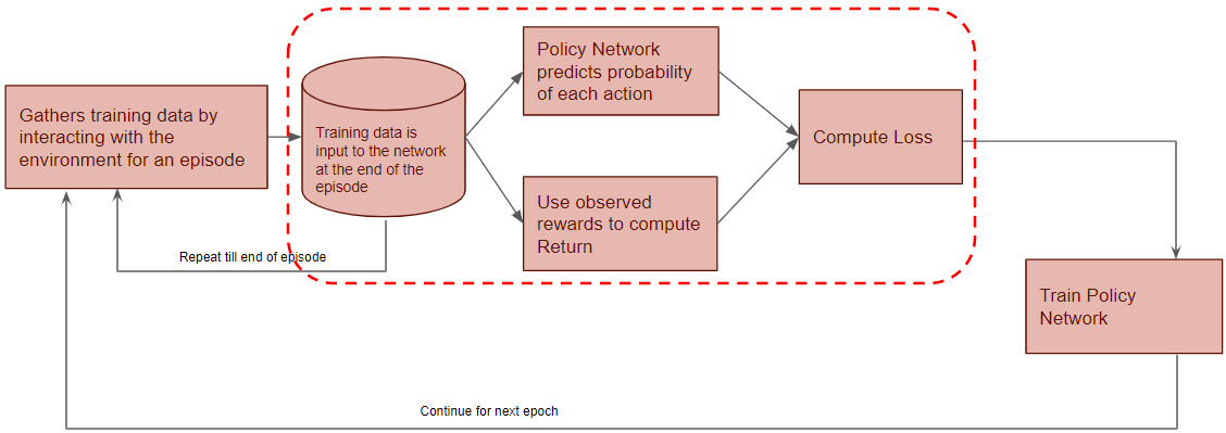
Now we’ll zoom in on the next phase of the flow.
 (Image by Author)
At the end of an episode, the training data is input to the Policy Network. It takes the current state and action from the data sample and predicts the probability of that action.
 (Image by Author)
The Discounted Return is calculated by taking the reward from the data sample.
 (Image by Author)
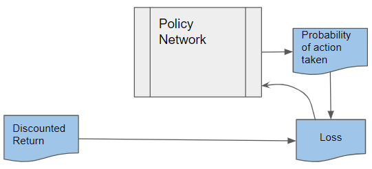
The discounted return and action probability are used to compute the Loss to train the Policy Network. The Policy Network learns to predict better actions until it finds the Optimal Policy.
 (Image by Author)
Policy-based solutions have some advantages over a Value-based solution
A Value-based solution learns a Value function that outputs the Q-value of all actions that can be taken from a state. They would struggle with problems where the number of actions is very large. For instance, you could have continuous actions (eg. a robot can rotate by any angle including fractional angles from 0 degrees to 360 degrees, raise its arm or turn its head by any angle, move at a speed which could be any real number between some range, and so on) which result in an infinite number of actions.
On the other hand, a Policy-based solution like Policy Gradient learns a policy function that outputs a probability distribution of actions, and therefore, they can handle problems with a large number of actions.
It also means that Policy Gradient can learn deterministic policies as well as stochastic policies, where there isn’t always a single best action. Since the agent picks an action by sampling from the probability distribution it can vary its actions each time.
On the other hand, with value-based solutions, the Optimal Policy is derived from the Optimal Q-value by picking the action with the highest Q-value. Thus they can learn only deterministic policies.
Finally, since policy-based methods find the policy directly, they are usually more efficient than value-based methods, in terms of training time.
Policy Gradient ensures adequate exploration
In contrast to value-based solutions which use an implicit ε-greedy policy, the Policy Gradient learns its policy as it goes.
At each step, it picks an action by sampling the predicted probability distribution. As a result it ends up taking a variety of different actions.
When training starts out, the probability distribution of actions that it outputs is fairly uniform since it doesn’t know which actions are preferred. This encourages exploration as it means that all actions are equally likely. As training progresses, the probability distribution converges on the best actions, thus maximizing exploitation. If there is only one best action for some state, then that probability distribution is a degenerate distribution resulting in a deterministic policy.
Policy Gradient Loss function
With Q-Learning and DQN, we had a target Q-value with which to compare our predicted Q-value. So it was fairly easy to define a Loss function for it. However, with Policy Gradient, there is no such target feature with which to compare its predicted action probability distribution.
All we have available is whether a selected action led to positive or negative rewards. How do we use this to define a Loss function in this case?
Let’s think about the objective that we want the Loss function to achieve. If an action results in a positive reward, we want that action to become more likely (ie. increase its probability) and if it results in a negative reward, we want that action to become less likely (ie. decrease its probability).
However, for a positive action, we don’t want to increase its probability to 1, which means that it becomes the only action to be taken, as the probability of all other actions would be reduced to 0. Similarly, for a negative action, we don’t want to reduce its probability to 0, which means that that action will never get taken. We want to continue exploring and trying different actions multiple times.
Instead, for a positive action, we want the probability to increase slightly while reducing the probability of all other actions slightly (since they all must sum to 1). This makes that action slightly more likely.
In other words, if we took action a1, and P(a) is the probability of taking action ‘a’, we want to maximize P(a1). Since Loss functions work by minimizing rather than maximizing, we can equivalently use 1 — P(a1) as our Loss. It approaches 0 as P(a1) approaches 1, so it encourages the network to modify its weights to adjust the probability distribution by increasing P(a1).
Similarly for a negative action.
Probability is represented as a floating point number and when those numbers are very small (near 0) or very large (near 1), these computations can cause numerical overflow problems.
To avoid this, we usually use -log (P(a1)) which behaves equivalently to 1 — P(a1). It also approaches 0 as P(a1) approaches 1, but ‘log’ does not suffer from overflow issues because those values have the advantage of having a broader range from (–∞,0) instead of (0, 1).
Finally, we do not want to assign equal weightage to every action. Those actions which resulted in more reward during the episode should get higher weightage. Therefore we use the Discounted Return of each action to determine its contribution. So the Loss function is -log (P(a)) * Rt, where Rt is the Discounted Return for action ‘a’. That way the probability of each action taken is updated in proportion to the Discounted Return resulting from that action.
Detailed Operation
Now let’s look at the detailed operation of the REINFORCE algorithm for Policy Gradients. From some initial starting state, the Policy Network takes the current state as input and outputs a probability distribution of all actions.
 (Image by Author)
We then pick an action by sampling from that distribution.
 (Image by Author)
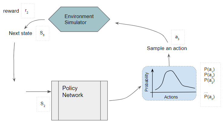
The action is fed to the environment which generates the Next state and reward. The Next state is fed back into the Policy Network.
 (Image by Author)
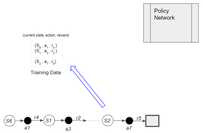
Each sample of observed experience is stored as training data. Note that the Policy Network weights remain fixed during this phase.
We continue doing this till the end of the episode. After that, we start the phase to train the Policy Network using the training data as input. The training batch holds an episode of samples.
 (Image by Author)
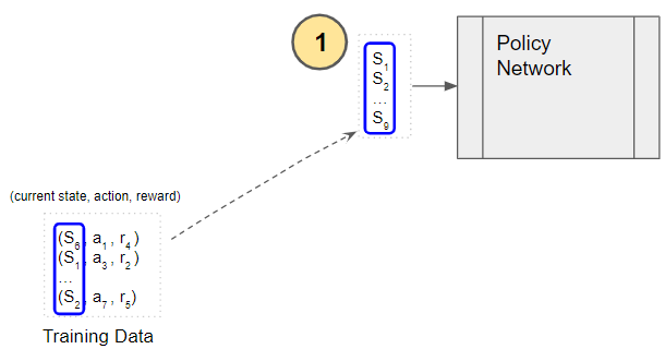
Each state that was visited in the episode is input to the Policy Network.
 (Image by Author)
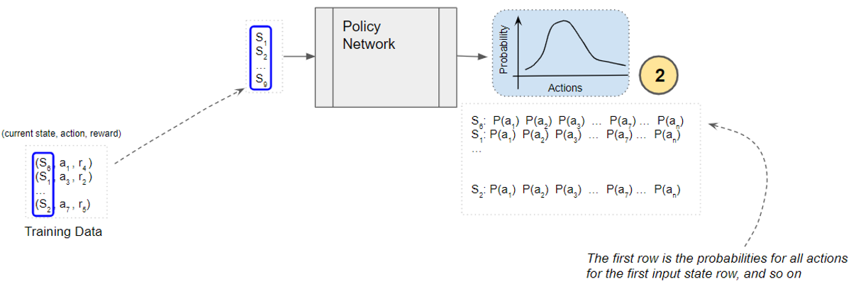
The Policy Network predicts the probability distribution of all actions from each of those states.
 (Image by Author)
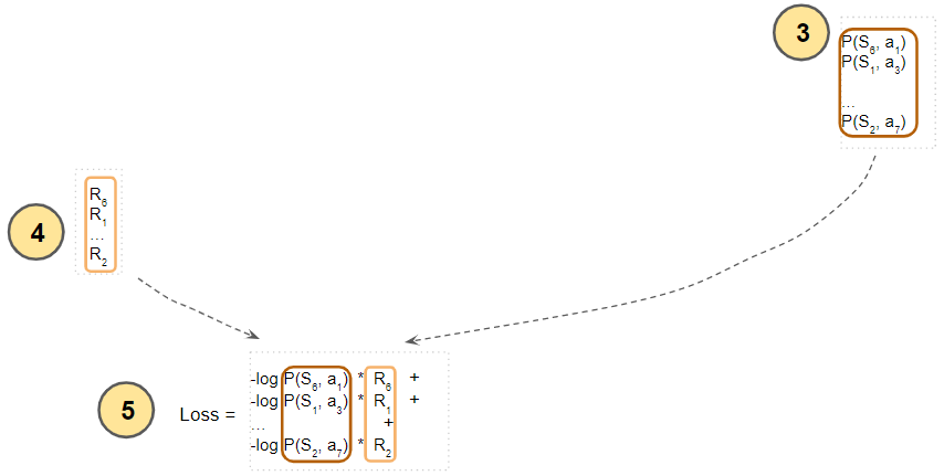
Get the probability of the action that was actually taken from each state.
 (Image by Author)
Compute the Discounted Return for each sample as the weighted sum of rewards.
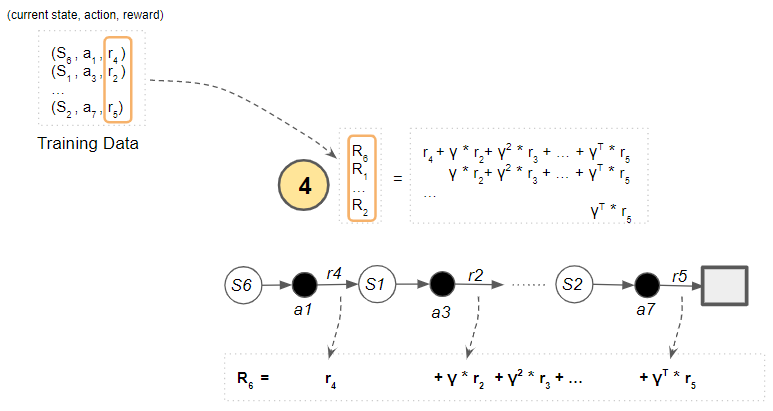 (Image by Author)
Then multiply the (log of) the action probability with the discounted return. We want to maximize this, but since neural nets work by minimizing a loss, we take its negative, which achieves the same effect. Finally, add up these negative quantities for all states.
 (Image by Author)
Putting it all together, here is the complete flow to compute the loss.
 (Image by Author)
This Loss is used to train the Policy Network, and then the cycle repeats for the next epoch.
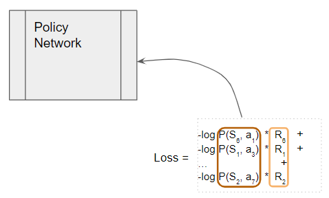 (Image by Author)
Conclusion We have now seen why the policy-based Policy Gradient method is used, and how the algorithm works. In the previous article, we had also seen the value-based DQN algorithm.
In the next article, we will finally learn about one of the more advanced RL solutions, known as Actor-Critic, which will build on the benefits of both of these approaches by combining them in an innovative way.
And finally, if you liked this article, you might also enjoy my other series on Transformers as well as Audio Deep Learning.
Transformers Explained Visually - Overview of functionality
Audio Deep Learning Made Simple - State-of-the-Art Techniques
Let’s keep learning!