This is the third article in my series on audio deep learning. So far we’ve learned how sound is represented digitally, and that deep learning architectures usually use a spectrogram of the sound. We’ve also seen how to pre-process audio data in Python to generate Mel Spectrograms.
In this article, we will take that a step further and enhance our Mel Spectrogram by tuning its hyper-parameters. We will also look at Augmentation techniques for audio data. Both of these are essential aspects of data preparation in order to get better performance from our audio deep learning models.
Here’s a quick summary of the articles I am planning in the series. My goal throughout will be to understand not just how something works but why it works that way.
- State-of-the-Art Techniques (What is sound and how it is digitized. What problems is audio deep learning solving in our daily lives. What are Spectrograms and why they are all-important.)
- Why Mel Spectrograms perform better (Processing audio data in Python. What are Mel Spectrograms and how to generate them)
- Feature Optimization and Augmentation — this article (Enhance Spectrograms features for optimal performance by hyper-parameter tuning and data augmentation)
- Audio Classification (End-to-end example and architecture to classify ordinary sounds. Foundational application for a range of scenarios.)
- Automatic Speech Recognition (Speech-to-Text algorithm and architecture, using CTC Loss and Decoding for aligning sequences.)
Spectrograms Optimization with Hyper-parameter tuning
In Part 2 we learned what a Mel Spectrogram is and how to create one using some convenient library functions. But to really get the best performance for our deep learning models, we should optimize the Mel Spectrograms for the problem that we’re trying to solve.
There are a number of hyper-parameters that we can use to tune how the Spectrogram is generated. For that, we need to understand a few concepts about how Spectrograms are constructed. (I’ll try to keep that as simple and intuitive as possible!)
Fast Fourier Transform (FFT)
One way to compute Fourier Transforms is by using a technique called DFT (Discrete Fourier Transform). The DFT is very expensive to compute, so in practice, the FFT (Fast Fourier Transform) algorithm is used, which is an efficient way to implement the DFT.
However, the FFT will give you the overall frequency components for the entire time series of the audio signal as a whole. It won’t tell you how those frequency components change over time within the audio signal. You will not be able to see, for example, that the first part of the audio had high frequencies while the second part had low frequencies, and so on.
Short-time Fourier Transform (STFT)
To get that more granular view and see the frequency variations over time, we use the STFT algorithm (Short-Time Fourier Transform). The STFT is another variant of the Fourier Transform that breaks up the audio signal into smaller sections by using a sliding time window. It takes the FFT on each section and then combines them. It is thus able to capture the variations of the frequency with time.
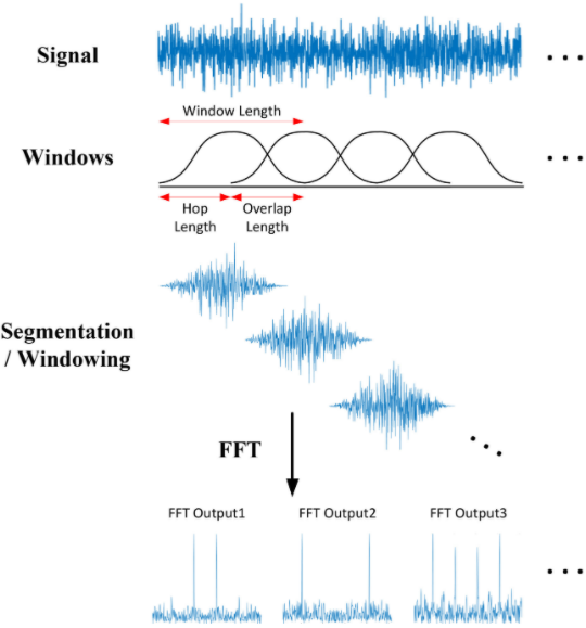 STFT slides an overlapping window along the signal and does a Fourier Transform on each segment (Source)
This splits the signal into sections along the Time axis. Secondly, it also splits the signal into sections along the Frequency axis. It takes the full range of frequencies and divides it up into equally spaced bands (in the Mel scale). Then, for each section of time, it calculates the Amplitude or energy for each frequency band.
Let’s make this clear with an example. We have a 1-minute audio clip that contains frequencies between 0Hz and 10000 Hz (in the Mel scale). Let’s say that the Mel Spectrogram algorithm:
- Chooses windows such that it splits our audio signal into 20 time-sections
- Decides to split our frequency range into 10 bands (ie. 0–1000Hz, 1000–2000Hz, … 9000–10000Hz).
The final output of the algorithm is a 2D Numpy array of shape (10, 20) where:
- Each of the 20 columns represents the FFT for one time-section.
- Each of the 10 rows represents Amplitude values for a frequency band.
Let’s take the first column, which is the FFT for the first time section. It has 10 rows.
- The first row is the Amplitude for the first frequency band between 0–1000 Hz.
- The second row is the Amplitude for the second frequency band between 1000–2000 Hz.
- … and so on.
Each column in the array becomes a ‘column’ in our Mel Spectrogram image.
Mel Spectrogram Hyperparameters
This gives us the hyperparameters for tuning our Mel Spectrogram. We’ll use the parameter names that Librosa uses. (Other libraries will have equivalent parameters)
Frequency Bands
- fmin — minimum frequency
- fmax — maximum frequency to display
- n_mels — number of frequency bands (ie. Mel bins). This is the height of the Spectrogram
Time Sections
- n_fft — window length for each time section
- hop_length — number of samples by which to slide the window at each step. Hence, the width of the Spectrogram is = Total number of samples / hop_length
You can adjust these hyperparameters based on the type of audio data that you have and the problem you’re solving.
MFCC (for Human Speech)
Mel Spectrograms work well for most audio deep learning applications. However, for problems dealing with human speech, like Automatic Speech Recognition, you might find that MFCC (Mel Frequency Cepstral Coefficients) sometimes work better.
These essentially take Mel Spectrograms and apply a couple of further processing steps. This selects a compressed representation of the frequency bands from the Mel Spectrogram that correspond to the most common frequencies at which humans speak.
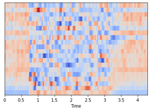 MFCC generated from audio (Image by Author)
Above, we had seen that the Mel Spectrogram for this same audio had shape (128, 134), whereas the MFCC has shape (20, 134). The MFCC extracts a much smaller set of features from the audio that are the most relevant in capturing the essential quality of the sound.
Data Augmentation
A common technique to increase the diversity of your dataset, particularly when you don’t have enough data, is to augment your data artificially. We do this by modifying the existing data samples in small ways.
For instance, with images, we might do things like rotate the image slightly, crop or scale it, modify colors or lighting, or add some noise to the image. Since the semantics of the image haven’t changed materially, so the same target label from the original sample will still apply to the augmented sample. eg. if the image was labeled as a ‘cat’, the augmented image will also be a ‘cat’.
But, from the model’s point of view, it feels like a new data sample. This helps your model generalize to a larger range of image inputs.
Just like with images, there are several techniques to augment audio data as well. This augmentation can be done both on the raw audio before producing the spectrogram, or on the generated spectrogram. Augmenting the spectrogram usually produces better results.
Spectrogram Augmentation
The normal transforms you would use for an image don’t apply to spectrograms. For instance, a horizontal flip or a rotation would substantially alter the spectrogram and the sound that it represents.
Instead, we use a method known as SpecAugment where we block out sections of the spectrogram. There are two flavors:
- Frequency mask — randomly mask out a range of consecutive frequencies by adding horizontal bars on the spectrogram.
- Time mask — similar to frequency masks, except that we randomly block out ranges of time from the spectrogram by using vertical bars.
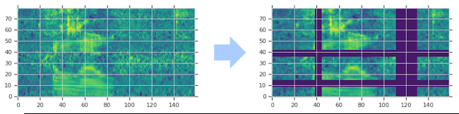 (Image by Author)
Raw Audio Augmentation
There are several options:
Time Shift — shift audio to the left or the right by a random amount.
- For sound such as traffic or sea waves which has no particular order, the audio could wrap around.
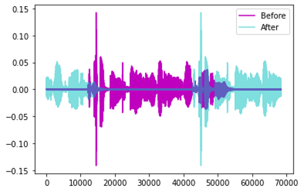 Augmentation by Time Shift (Image by Author)
- Alternately, for sounds such as human speech where the order does matter, the gaps can be filled with silence.
Pitch Shift — randomly modify the frequency of parts of the sound.
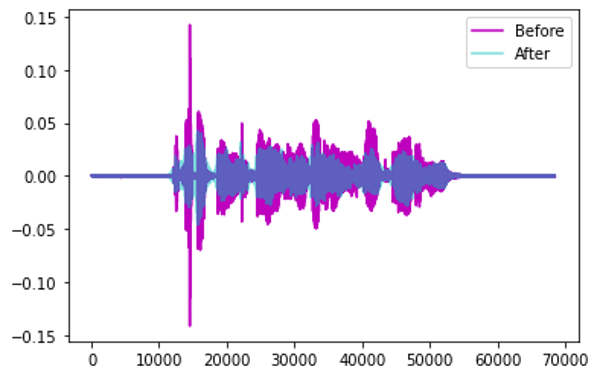 Augmentation by Pitch Shift (Image by Author)
Time Stretch — randomly slow down or speed up the sound.
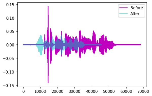 Augmentation by Time Stretch (Image by Author)
Add Noise — add some random values to the sound.
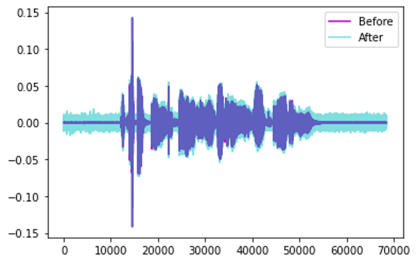 Augmentation by Adding Noise (Image by Author)
Conclusion
We have now seen how we pre-process and prepare audio data for input to deep learning models. These approaches are commonly applied for a majority of audio applications.
We are now ready to explore some real deep learning applications and will cover an Audio Classification example in the next article, where we’ll see these techniques in action.
And finally, if you liked this article, you might also enjoy my other series on Transformers as well as Reinforcement Learning.
Transformers Explained Visually: Overview of functionality
Reinforcement Learning Made Simple (Part 1): Intro to Basic Concepts and Terminology
Let’s keep learning!