Audio Deep Learning Made Simple - Sound Classification, Step-by-Step

Sound Classification is one of the most widely used applications in Audio Deep Learning. It involves learning to classify sounds and to predict the category of that sound. This type of problem can be applied to many practical scenarios e.g. classifying music clips to identify the genre of the music, or classifying short utterances by a set of speakers to identify the speaker based on the voice.

In this article, we will walk through a simple demo application so as to understand the approach used to solve such audio classification problems. My goal throughout will be to understand not just how something works but why it works that way.

I have a few more articles in my audio deep learning series that you might find useful. They explore other fascinating topics in this space including how we prepare audio data for deep learning, why we use Mel Spectrograms for deep learning models and how they are generated and optimized.

State-of-the-Art Techniques (What is sound and how it is digitized. What problems is audio deep learning solving in our daily lives. What are Spectrograms and why they are all-important.)
Why Mel Spectrograms perform better (Processing audio data in Python. What are Mel Spectrograms and how to generate them)
Feature Optimization and Augmentation (Enhance Spectrograms features for optimal performance by hyper-parameter tuning and data augmentation)
Audio Classification — this article (End-to-end example and architecture to classify ordinary sounds. Foundational application for a range of scenarios.)
Automatic Speech Recognition (Speech-to-Text algorithm and architecture, using CTC Loss and Decoding for aligning sequences.)

Audio Classification

Just like classifying hand-written digits using the MNIST dataset is considered a ‘Hello World”-type problem for Computer Vision, we can think of this application as the introductory problem for audio deep learning.

We will start with sound files, convert them into spectrograms, input them into a CNN plus Linear Classifier model, and produce predictions about the class to which the sound belongs.

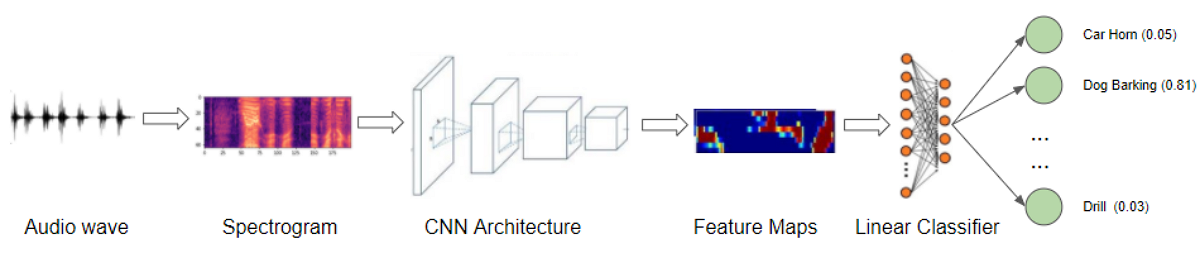Audio Classification application (Image by Author)

There are many suitable datasets available for sounds of different types. These datasets contain a large number of audio samples, along with a class label for each sample that identifies what type of sound it is, based on the problem you are trying to address.

These class labels can often be obtained from some part of the filename of the audio sample or from the sub-folder name in which the file is located. Alternately the class labels are specified in a separate metadata file, usually in TXT, JSON, or CSV format.

Example problem — Classifying ordinary city sounds

For our demo, we will use the Urban Sound 8K dataset that consists of a corpus of ordinary sounds recorded from day-to-day city life. The sounds are taken from 10 classes such as drilling, dogs barking, and sirens. Each sound sample is labeled with the class to which it belongs.

After downloading the dataset, we see that it consists of two parts:

Audio files in the ‘audio’ folder: It has 10 sub-folders named ‘fold1’ through ‘fold10’. Each sub-folder contains a number of ‘.wav’ audio samples eg. ‘fold1/103074–7–1–0.wav’
Metadata in the ‘metadata’ folder: It has a file ‘UrbanSound8K.csv’ that contains information about each audio sample in the dataset such as its filename, its class label, the ‘fold’ sub-folder location, and so on. The class label is a numeric Class ID from 0–9 for each of the 10 classes. eg. the number 0 means air conditioner, 1 is a car horn, and so on.

The samples are around 4 seconds in length. Here’s what one sample looks like:

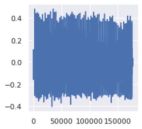An audio sample of a drill (Image by Author)

Sample Rate, Number of Channels, Bits, and Audio Encoding

The recommendation of the dataset creators is to use the folds for doing 10-fold cross-validation to report metrics and evaluate the performance of your model. However, since our goal in this article is primarily as a demo of an audio deep learning example rather than to obtain the best metrics, we will ignore the folds and treat all the samples simply as one large dataset.

Prepare training data

As for most deep learning problems, we will follow these steps:

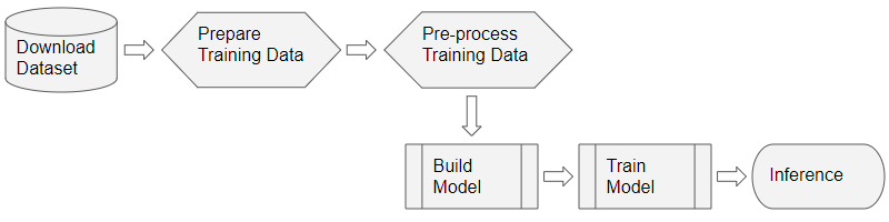Deep Learning Workflow (Image by Author)

The training data for this problem will be fairly simple:

The features (X) are the audio file paths
The target labels (y) are the class names

Since the dataset has a metadata file that contains this information already, we can use that directly. The metadata contains information about each audio file.

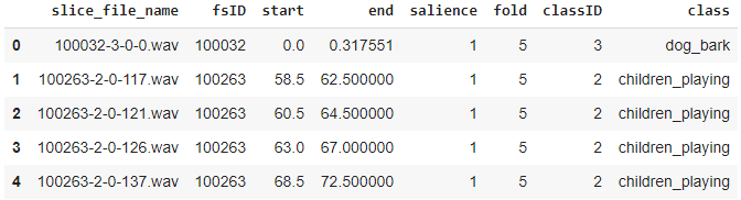
Since it is a CSV file, we can use Pandas to read it. We can prepare the feature and label data from the metadata.

This gives us the information we need for our training data.

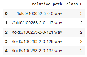Training data with audio file paths and class IDs

Scan the audio file directory when metadata isn’t available

Having the metadata file made things easy for us. How would we prepare our data for datasets that do not contain a metadata file?

Many datasets consist of only audio files arranged in a folder structure from which class labels can be derived. To prepare our training data in this format, we would do the following:

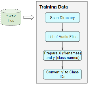Preparing Training Data when metadata isn’t available (Image by Author)

Scan the directory and prepare a list of all the audio file paths.
Extract the class label from each file name, or from the name of the parent sub-folder
Map each class name from text to a numeric class ID

With or without metadata, the result would be the same — features consisting of a list of audio file names and target labels consisting of class IDs.

Audio Pre-processing: Define Transforms

This training data with audio file paths cannot be input directly into the model. We have to load the audio data from the file and process it so that it is in a format that the model expects.

This audio pre-processing will all be done dynamically at runtime when we will read and load the audio files. This approach is similar to what we would do with image files as well. Since audio data, like image data, can be fairly large and memory-intensive, we don’t want to read the entire dataset into memory all at once, ahead of time. So we keep only the audio file names (or image file names) in our training data.

Then, at runtime, as we train the model one batch at a time, we will load the audio data for that batch and process it by applying a series of transforms to the audio. That way we keep audio data for only one batch in memory at a time.

With image data, we might have a pipeline of transforms where we first read the image file as pixels and load it. Then we might apply some image processing steps to reshape and resize the data, crop them to a fixed size and convert them into grayscale from RGB. We might also apply some image augmentation steps like rotation, flips, and so on.

The processing for audio data is very similar. Right now we’re only defining the functions, they will be run a little later when we feed data to the model during training.

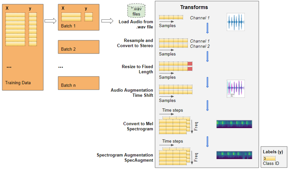
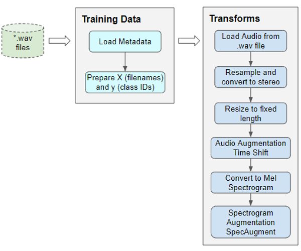Pre-processing the training data for input to our model (Image by Author)

Read audio from a file

The first thing we need is to read and load the audio file in “.wav” format. Since we are using Pytorch for this example, the implementation below uses torchaudio for the audio processing, but librosa will work just as well.

Audio wave loaded from a file (Image by Author)

Convert to two channels

Some of the sound files are mono (ie. 1 audio channel) while most of them are stereo (ie. 2 audio channels). Since our model expects all items to have the same dimensions, we will convert the mono files to stereo, by duplicating the first channel to the second.

Standardize sampling rate

Some of the sound files are sampled at a sample rate of 48000Hz, while most are sampled at a rate of 44100Hz. This means that 1 second of audio will have an array size of 48000 for some sound files, while it will have a smaller array size of 44100 for the others. Once again, we must standardize and convert all audio to the same sampling rate so that all arrays have the same dimensions.

Resize to the same length

We then resize all the audio samples to have the same length by either extending its duration by padding it with silence, or by truncating it. We add that method to our AudioUtil class.

Data Augmentation: Time Shift

Next, we can do data augmentation on the raw audio signal by applying a Time Shift to shift the audio to the left or the right by a random amount. I go into a lot more detail about this and other data augmentation techniques in this article.

Time Shift of the audio wave (Image by Author)

Mel Spectrogram

We then convert the augmented audio to a Mel Spectrogram. They capture the essential features of the audio and are often the most suitable way to input audio data into deep learning models. To get more background about this, you might want to read my articles (here and here) which explain in simple words what a Mel Spectrogram is, why they are crucial for audio deep learning, as well as how they are generated and how to tune them for getting the best performance from your models.

Mel Spectrogram of an audio wave (Image by Author)

Data Augmentation: Time and Frequency Masking

Now we can do another round of augmentation, this time on the Mel Spectrogram rather than on the raw audio. We will use a technique called SpecAugment that uses these two methods:

Frequency mask — randomly mask out a range of consecutive frequencies by adding horizontal bars on the spectrogram.
Time mask — similar to frequency masks, except that we randomly block out ranges of time from the spectrogram by using vertical bars.

Mel Spectrogram after SpecAugment. Notice the horizontal and vertical mask bands (Image by Author)

Define Custom Data Loader

Now that we have defined all the pre-processing transform functions we will define a custom Pytorch Dataset object.

To feed your data to a model with Pytorch, we need two objects:

A custom Dataset object that uses all the audio transforms to pre-process an audio file and prepares one data item at a time.
A built-in DataLoader object that uses the Dataset object to fetch individual data items and packages them into a batch of data.

Prepare Batches of Data with the Data Loader

All of the functions we need to input our data to the model have now been defined.

We use our custom Dataset to load the Features and Labels from our Pandas dataframe and split that data randomly in an 80:20 ratio into training and validation sets. We then use them to create our training and validation Data Loaders.

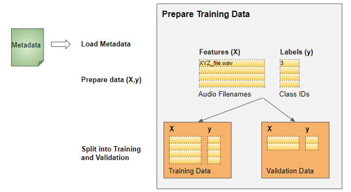Split our data for training and validation (Image by Author)

When we start training, the Data Loader will randomly fetch one batch of input Features containing the list of audio file names and run the pre-processing audio transforms on each audio file. It will also fetch a batch of the corresponding target Labels containing the class IDs. Thus it will output one batch of training data at a time, which can directly be fed as input to our deep learning model.

Data Loader applies transforms and prepares one batch of data at a time (Image by Author)

Let’s walk through the steps as our data gets transformed, starting with an audio file:

The audio from the file gets loaded into a Numpy array of shape (num_channels, num_samples). Most of the audio is sampled at 44.1kHz and is about 4 seconds in duration, resulting in 44,100 * 4 = 176,400 samples. If the audio has 1 channel, the shape of the array will be (1, 176,400). Similarly, audio of 4 seconds duration with 2 channels and sampled at 48kHz will have 192,000 samples and a shape of (2, 192,000).
Since the channels and sampling rates of each audio are different, the next two transforms resample the audio to a standard 44.1kHz and to a standard 2 channels.
Since some audio clips might be more or less than 4 seconds, we also standardize the audio duration to a fixed length of 4 seconds. Now arrays for all items have the same shape of (2, 176,400)
The Time Shift data augmentation now randomly shifts each audio sample forward or backward. The shapes are unchanged.
The augmented audio is now converted into a Mel Spectrogram, resulting in a shape of (num_channels, Mel freq_bands, time_steps) = (2, 64, 344)
The SpecAugment data augmentation now randomly applies Time and Frequency Masks to the Mel Spectrograms. The shapes are unchanged.

Thus, each batch will have two tensors, one for the X feature data containing the Mel Spectrograms and the other for the y target labels containing numeric Class IDs. The batches are picked randomly from the training data for each training epoch.

Each batch has a shape of (batch_sz, num_channels, Mel freq_bands, time_steps)

A batch of (X, y) data

We can visualize one item from the batch. We see the Mel Spectrogram with vertical and horizontal stripes showing the Frequency and Time Masking data augmentation.

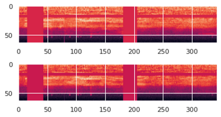A batch of (X, y) data

The data is now ready for input to the model.

Create Model

The data processing steps that we just did are the most unique aspects of our audio classification problem. From here on, the model and training procedure are quite similar to what is commonly used in a standard image classification problem and are not specific to audio deep learning.

Since our data now consists of Spectrogram images, we build a CNN classification architecture to process them. It has four convolutional blocks which generate the feature maps. That data is then reshaped into the format we need so it can be input into the linear classifier layer, which finally outputs the predictions for the 10 classes.

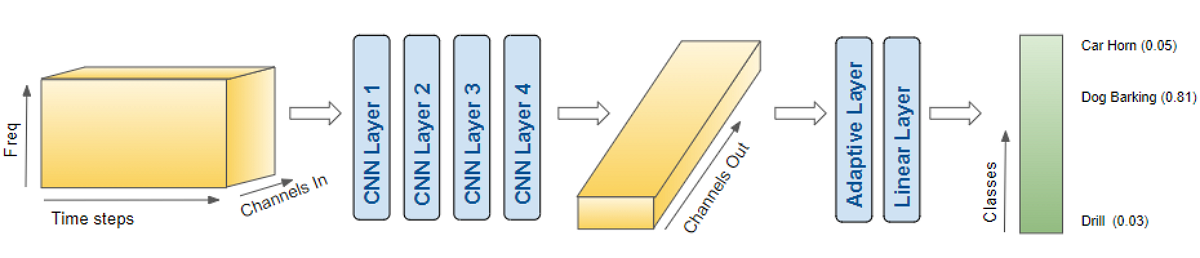The model takes a batch of pre-processed data and outputs class predictions (Image by Author)

A few more details about how the model processes a batch of data:

A batch of images is input to the model with shape (batch_sz, num_channels, Mel freq_bands, time_steps) ie. (16, 2, 64, 344).
Each CNN layer applies its filters to step up the image depth ie. number of channels. The image width and height are reduced as the kernels and strides are applied. Finally, after passing through the four CNN layers, we get the output feature maps ie. (16, 64, 4, 22).
This gets pooled and flattened to a shape of (16, 64) and then input to the Linear layer.
The Linear layer outputs one prediction score per class ie. (16, 10)

Training

We are now ready to create the training loop to train the model.

We define the functions for the optimizer, loss, and scheduler to dynamically vary our learning rate as training progresses, which usually allows training to converge in fewer epochs.

We train the model for several epochs, processing a batch of data in each iteration. We keep track of a simple accuracy metric which measures the percentage of correct predictions.

Inference

Ordinarily, as part of the training loop, we would also evaluate our metrics on the validation data. We would then do inference on unseen data, perhaps by keeping aside a test dataset from the original data. However, for the purposes of this demo, we will use the validation data for this purpose.

We run an inference loop taking care to disable the gradient updates. The forward pass is executed with the model to get predictions, but we do not need to backpropagate or run the optimizer.

Conclusion

We have now seen an end-to-end example of sound classification which is one of the most foundational problems in audio deep learning. Not only is this used in a wide range of applications, but many of the concepts and techniques that we covered here will be relevant to more complicated audio problems such as automatic speech recognition where we start with human speech, understand what people are saying, and convert it to text.

And finally, if you liked this article, you might also enjoy my other series on Transformers as well as Reinforcement Learning.

Transformers Explained Visually: Overview of functionality

Reinforcement Learning Made Simple (Part 1): Intro to Basic Concepts and Terminology

Let’s keep learning!