Audio Deep Learning Made Simple - Why Mel Spectrograms perform better

This is the second article in my series on audio deep learning. Now that we know how sound is represented digitally, and that we need to convert it into a spectrogram for use in deep learning architectures, let us understand in more detail how that is done and how we can tune that conversion to get better performance.

Since data preparation is so critical, particularly in the case of audio deep learning models, that will be the focus of the next two articles.

Here’s a quick summary of the articles I am planning in the series. My goal throughout will be to understand not just how something works but why it works that way.

1. State-of-the-Art Techniques (What is sound and how it is digitized. What problems is audio deep learning solving in our daily lives. What are Spectrograms and why they are all-important.)
2. Why Mel Spectrograms perform better — this article (Processing audio data in Python. What are Mel Spectrograms and how to generate them)
3. Feature Optimization and Augmentation (Enhance Spectrograms features for optimal performance by hyper-parameter tuning and data augmentation)
4. Audio Classification (End-to-end example and architecture to classify ordinary sounds. Foundational application for a range of scenarios.)
5. Automatic Speech Recognition (Speech-to-Text algorithm and architecture, using CTC Loss and Decoding for aligning sequences.)

Audio File Formats and Python Libraries

Audio data for your deep learning models will usually start out as digital audio files. From listening to sound recordings and music, we all know that these files are stored in a variety of formats based on how the sound is compressed. Examples of these formats are .wav, .mp3, .wma, .aac, .flac and many more.

Python has some great libraries for audio processing. Librosa is one of the most popular and has an extensive set of features. scipy is also commonly used. If you are using Pytorch, it has a companion library called torchaudio that is tightly integrated with Pytorch. It doesn’t have as much functionality as Librosa, but it is built specifically for deep learning.

They all let you read audio files in different formats. The first step is to load the file. With librosa:

Or, you can also do the same thing using scipy:

You can then visualize the sound wave:

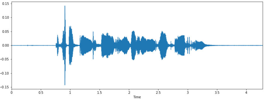Visualize the sound wave (Image by Author)

And listen to it. If you are using a Jupyter notebook, you can play the audio directly in a cell.

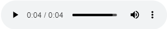Play audio in a notebook cell (Image by Author)

Audio Signal Data

As we saw in the previous article, audio data is obtained by sampling the sound wave at regular time intervals and measuring the intensity or amplitude of the wave at each sample. The metadata for that audio tells us the sampling rate which is the number of samples per second.

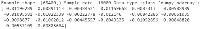
When that audio is saved in a file it is in a compressed format. When the file is loaded, it is decompressed and converted into a Numpy array. This array looks the same no matter which file format you started with.

In memory, audio is represented as a time series of numbers, representing the amplitude at each timestep. For instance, if the sample rate was 16800, a one-second clip of audio would have 16800 numbers. Since the measurements are taken at fixed intervals of time, the data contains only the amplitude numbers and not the time values. Given the sample rate, we can figure out at what time instant each amplitude number measurement was taken.

The bit-depth tells us how many possible values those amplitude measurements for each sample can take. For example, a bit-depth of 16 means that the amplitude number can be between 0 and 65535 (2 ¹⁶ — 1). The bit-depth influences the resolution of the audio measurement — the higher the bit-depth, the better the audio fidelity.

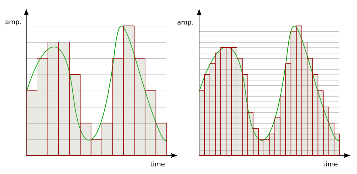Bit-depth and sample-rate determine the audio resolution (Source)

Spectrograms

Deep learning models rarely take this raw audio directly as input. As we learned in Part 1, the common practice is to convert the audio into a spectrogram. The spectrogram is a concise ‘snapshot’ of an audio wave and since it is an image, it is well suited to being input to CNN-based architectures developed for handling images.

Spectrograms are generated from sound signals using Fourier Transforms. A Fourier Transform decomposes the signal into its constituent frequencies and displays the amplitude of each frequency present in the signal.

A Spectrogram chops up the duration of the sound signal into smaller time segments and then applies the Fourier Transform to each segment, to determine the frequencies contained in that segment. It then combines the Fourier Transforms for all those segments into a single plot.

It plots Frequency (y-axis) vs Time (x-axis) and uses different colors to indicate the Amplitude of each frequency. The brighter the color the higher the energy of the signal.

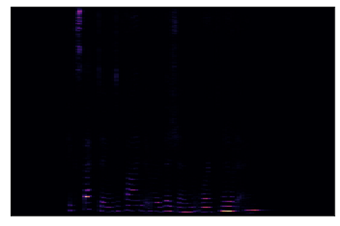Simple Spectrogram (Image by Author)

Unfortunately, when we display this spectrogram there isn’t much information for us to see. What happened to all those colorful spectrograms we used to see in Science class?

This happens because of the way humans perceive sound. Most of what we are able to hear are concentrated in a narrow range of frequencies and amplitudes. Let’s explore that first so we can figure out how to produce those lovely spectrograms.

How do humans hear frequencies?

The way we hear frequencies in sound is known as ‘pitch’. It is a subjective impression of the frequency. So a high-pitched sound has a higher frequency than a low-pitched sound. Humans do not perceive frequencies linearly. We are more sensitive to differences between lower frequencies than higher frequencies.

For instance, if you listened to different pairs of sound as follows:

• 100Hz and 200Hz
• 1000Hz and 1100Hz
• 10000Hz and 10100 Hz

What is your perception of the “distance” between each pair of sounds? Are you able to tell each pair of sounds apart?

Even though in all cases, the actual frequency difference between each pair is exactly the same at 100 Hz, the pair at 100Hz and 200Hz will sound further apart than the pair at 1000Hz and 1100Hz. And you will hardly be able to distinguish between the pair at 10000Hz and 10100Hz.

However, this may seem less surprising if we realize that the 200Hz frequency is actually double the 100Hz, whereas the 10100Hz frequency is only 1% higher than the 10000Hz frequency.

This is how humans perceive frequencies. We hear them on a logarithmic scale rather than a linear scale. How do we account for this in our data?

Mel Scale

The Mel Scale was developed to take this into account by conducting experiments with a large number of listeners. It is a scale of pitches, such that each unit is judged by listeners to be equal in pitch distance from the next.

Mel Scale measures human perception of pitch (Source, by permission of Prof Barry Truax)

How do humans hear amplitudes?

The human perception of the amplitude of a sound is its loudness. And similar to frequency, we hear loudness logarithmically rather than linearly. We account for this using the Decibel scale.

Decibel Scale

On this scale, 0 dB is total silence. From there, measurement units increase exponentially. 10 dB is 10 times louder than 0 dB, 20 dB is 100 times louder and 30 dB is 1000 times louder. On this scale, a sound above 100 dB starts to become unbearably loud.

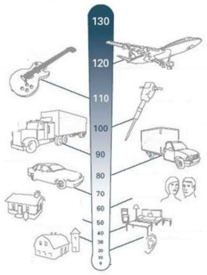Decibel levels of common sounds (Adapted from Source)

We can see that, to deal with sound in a realistic manner, it is important for us to use a logarithmic scale via the Mel Scale and the Decibel Scale when dealing with Frequencies and Amplitudes in our data.

That is exactly what the Mel Spectrogram is intended to do.

Mel Spectrograms

A Mel Spectrogram makes two important changes relative to a regular Spectrogram that plots Frequency vs Time.

• It uses the Mel Scale instead of Frequency on the y-axis.
• It uses the Decibel Scale instead of Amplitude to indicate colors.

For deep learning models, we usually use this rather than a simple Spectrogram.

Let’s modify our Spectrogram code above to use the Mel Scale in place of Frequency.

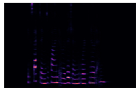Spectrogram using Mel Scale (Image by Author)

This is better than before, but most of the spectrogram is still dark and not carrying enough useful information. So let’s modify it to use the Decibel Scale instead of Amplitude.

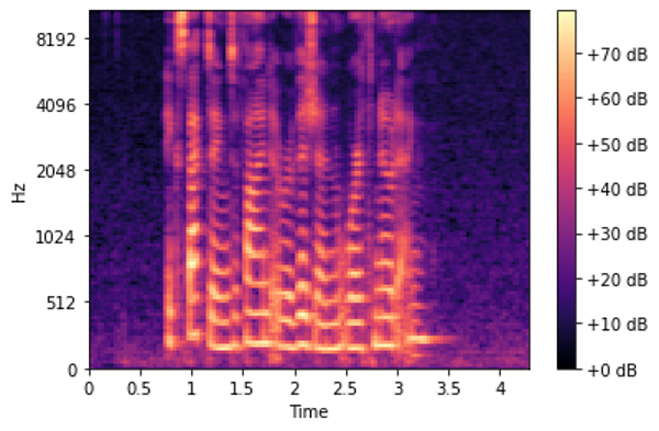Mel Spectrogram (Image by Author)

Finally! This is what we were really looking for 😃.

Conclusion

We have now seen how we pre-process audio data and prepare Mel Spectrograms. But before we can input them into deep learning models, we have to optimize them to obtain the best performance.

In the next article, we will look at how we can enhance the data for our models by tuning our Mel Spectrograms, as well as augmenting our audio data to help our models generalize to a wider range of inputs.

And finally, if you liked this article, you might also enjoy my other series on Transformers as well as Reinforcement Learning.

Transformers Explained Visually: Overview of functionality

Reinforcement Learning Made Simple (Part 1): Intro to Basic Concepts and Terminology

Let’s keep learning!