This is the fifth article in my series on Reinforcement Learning (RL). We now have a good understanding of the concepts that form the building blocks of an RL problem, and the techniques used to solve them. We have also taken a detailed look at the Q-Learning algorithm which forms the foundation of Deep Q Networks (DQN) which is the focus of this article.
With DQNs, we are finally able to being our journey into Deep Reinforcement Learning which is perhaps the most innovative area of Reinforcement Learning today. We’ll go through this algorithm step-by-step including some of the game-changing innovations like Experience Replay to understand exactly how they helped DQNs achieve their world-beating results when they were first introduced.
Here’s a quick summary of the previous and following articles in the series. My goal throughout will be to understand not just how something works but why it works that way.
- Intro to Basic Concepts and Terminology (What is an RL problem, and how to apply an RL problem-solving framework to it using techniques from Markov Decision Processes and concepts such as Return, Value, and Policy)
- Solution Approaches (Overview of popular RL solutions, and categorizing them based on the relationship between these solutions. Important takeaways from the Bellman equation, which is the foundation for all RL algorithms.)
- Model-free algorithms (Similarities and differences of Value-based and Policy-based solutions using an iterative algorithm to incrementally improve predictions. Exploitation, Exploration, and ε-greedy policies.)
- Q-Learning (In-depth analysis of this algorithm, which is the basis for subsequent deep-learning approaches. Develop intuition about why this algorithm converges to the optimal values.)
- Deep Q Networks — this article (Our first deep-learning algorithm. A step-by-step walkthrough of exactly how it works, and why those architectural choices were made.)
- Policy Gradient (Our first policy-based deep-learning algorithm.)
- Actor-Critic (Sophisticated deep-learning algorithm which combines the best of Deep Q Networks and Policy Gradients.)
If you haven’t read the earlier articles, particularly the fourth one on Q-Learning, it would be a good idea to read them first, as this article builds on many of the concepts that we discussed there.
Overview of Deep Q Networks
Q-table can handle simple problems with few states
Q Learning builds a Q-table of State-Action values, with dimension (s, a), where s is the number of states and a is the number of actions. Fundamentally, a Q-table maps state and action pairs to a Q-value.
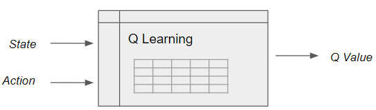 Q Learning looks up state-action pairs in a Q table (Image by Author)
However, in a real-world scenario, the number of states could be huge, making it computationally intractable to build a table.
Use a Q-Function for real-world problems
To address this limitation we use a Q-function rather than a Q-table, which achieves the same result of mapping state and action pairs to a Q value.
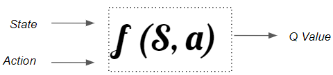 A state-action function is required to handle real-world scenarios with a large state space. (Image by Author)
Neural Nets are the best Function Approximators
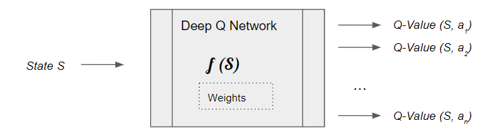
Since neural networks are excellent at modeling complex functions, we can use a neural network, which we call a Deep Q Network, to estimate this Q function.
This function maps a state to the Q values of all the actions that can be taken from that state.
 (Image by Author)
It learns the network’s parameters (weights) such that it can output the Optimal Q values.
The underlying principle of a Deep Q Network is very similar to the Q Learning algorithm. It starts with arbitrary Q-value estimates and explores the environment using the ε-greedy policy. And at its core, it uses the same notion of dual actions, a current action with a current Q-value and a target action with a target Q-value, for its update logic to improve its Q-value estimates.
DQN Architecture Components
The DQN architecture has two neural nets, the Q network and the Target networks, and a component called Experience Replay. The Q network is the agent that is trained to produce the Optimal State-Action value.
Experience Replay interacts with the environment to generate data to train the Q Network.
 (Image by Author)
The Q Network is a fairly standard neural network architecture and could be as simple as a linear network with a couple of hidden layers if your state can be represented via a set of numeric variables. Or if your state data is represented as images or text, you might use a regular CNN or RNN architecture.
The Target network is identical to the Q network.
High-level DQN Workflow
The DQN gets trained over multiple time steps over many episodes. It goes through a sequence of operations in each time step:
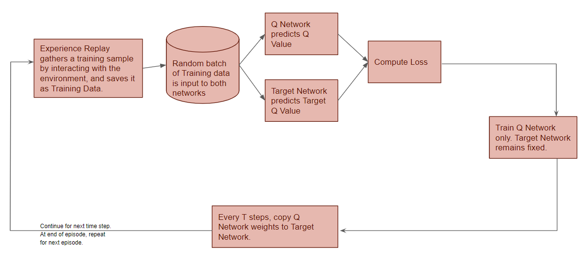 These operations are performed in each time-step (Image by Author)
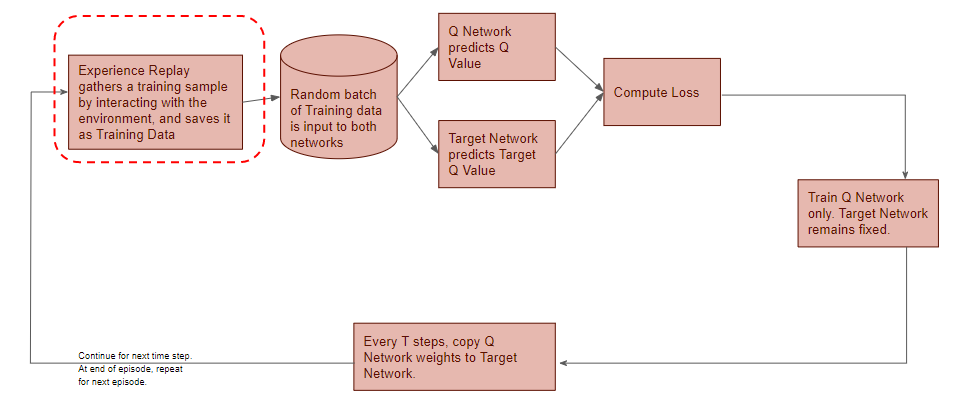
Gather Training Data
Now let’s zoom in on this first phase.
 (Image by Author)
Experience Replay selects an ε-greedy action from the current state, executes it in the environment, and gets back a reward and the next state.
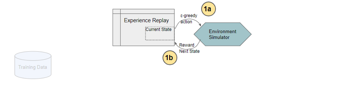 (Image by Author)
It saves this observation as a sample of training data.
 (Image by Author)
Next, we’ll zoom in on the next phase of the flow.
 (Image by Author)
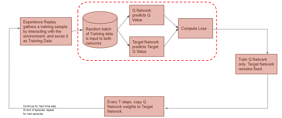
Q Network predicts Q-value
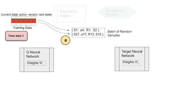
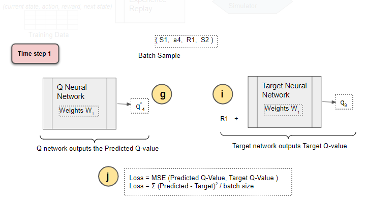
All prior Experience Replay observations are saved as training data. We now take a random batch of samples from this training data, so that it contains a mix of older and more recent samples.
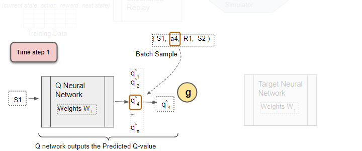
This batch of training data is then inputted to both networks. The Q network takes the current state and action from each data sample and predicts the Q value for that particular action. This is the ‘Predicted Q Value’.
 (Image by Author)
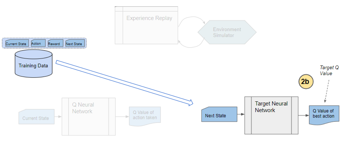
Target Network predicts Target Q-value
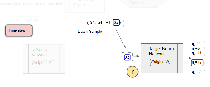
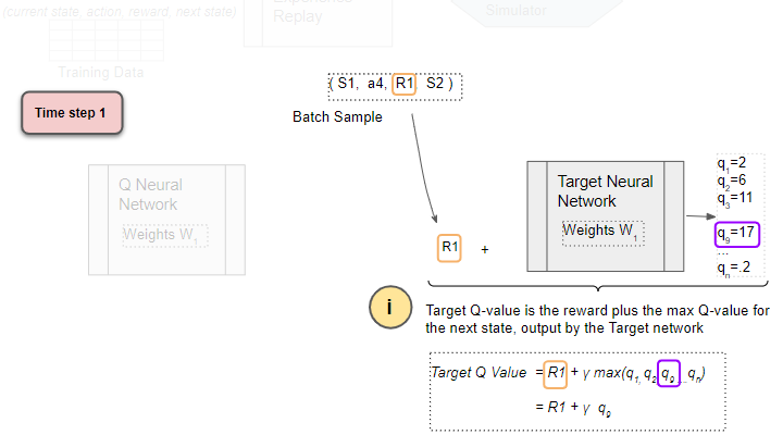
The Target network takes the next state from each data sample and predicts the best Q value out of all actions that can be taken from that state. This is the ‘Target Q Value’.
 (Image by Author)
Compute Loss and Train Q Network
The Predicted Q Value, Target Q Value, and the observed reward from the data sample is used to compute the Loss to train the Q Network. The Target Network is not trained.
 (Image by Author)
Why do we need Experience Replay?
You are probably wondering why we need a separate Experience Replay memory at all? Why don’t we simply take an action, observe results from the environment, and then feed that data to the Q Network?
The answer to that is straightforward. We know that neural networks typically take a batch of data. If we trained it with single samples, each sample and the corresponding gradients would have too much variance, and the network weights would never converge.
Alright, in that case, the obvious answer is why don’t we take a few actions in sequence one after the other and then feed that data as a batch to the Q Network? That should help to smoothen out the noise and result in more stable training, shouldn’t it?
Here the answer is much more subtle. Recall that when we train neural networks, a best practice is to select a batch of samples after shuffling the training data randomly. This ensures that there is enough diversity in the training data to allow the network to learn meaningful weights that generalize well and can handle a range of data values.
Would that occur if we passed a batch of data from sequential actions? Let’s take a scenario of a robot learning to navigate a factory floor. Let’s say that at a certain point in time, it is trying to find its way around a particular corner of the factory. All of the actions that it would take over the next few moves would be confined to that section of the factory.
If the network tried to learn from that batch of actions, it would update its weights to deal specifically with that location in the factory. But it would not learn anything about other parts of the factory. If sometime later, the robot moves to another location, all of its actions and hence the network’s learnings for a while would be narrowly focused on that new location. It might then undo what it had learned from the original location.
Hopefully, you’re starting to see the problem here. Sequential actions are highly correlated with one another and are not randomly shuffled, as the network would prefer. This results in a problem called Catastrophic Forgetting where the network unlearns things that it had learned a short while earlier.
This is why the Experience Replay memory was introduced. All of the actions and observations that the agent has taken from the beginning (limited by the capacity of the memory, of course) are stored. Then a batch of samples is randomly selected from this memory. This ensures that the batch is ‘shuffled’ and contains enough diversity from older and newer samples (eg. from several regions of the factory floor and under different conditions) to allow the network to learn weights that generalize to all the scenarios that it will be required to handle.
Why do we need a second neural network (Target Network)?
The second puzzling thing is why we need a second neural network? And that network is not getting trained, so that makes it all the more puzzling.
Firstly, it is possible to build a DQN with a single Q Network and no Target Network. In that case, we do two passes through the Q Network, first to output the Predicted Q value, and then to output the Target Q value.
But that could create a potential problem. The Q Network’s weights get updated at each time step, which improves the prediction of the Predicted Q value. However, since the network and its weights are the same, it also changes the direction of our predicted Target Q values. They do not remain steady but can fluctuate after each update. This is like chasing a moving target 😄.
By employing a second network that doesn’t get trained, we ensure that the Target Q values remain stable, at least for a short period. But those Target Q values are also predictions after all and we do want them to improve, so a compromise is made. After a pre-configured number of time-steps, the learned weights from the Q Network are copied over to the Target Network.
It has been found that using a Target Network results in more stable training.
DQN Operation in depth
Now that we understand the overall flow, let’s look at the detailed operation of the DQN. First, the network is initialized.
Initialization
Execute a few actions with the environment to bootstrap the replay data.
 (Image by Author)
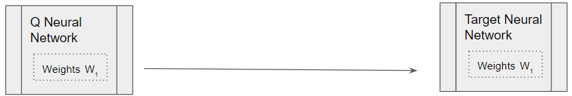
Initialize the Q Network with random weights and copy them to the Target Network.
 (Image by Author)
Experience Replay
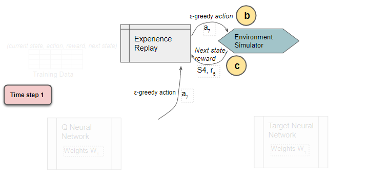
Starting with the first time step, the Experience Replay starts the training data generation phase and uses the Q Network to select an ε-greedy action. The Q Network acts as the agent while interacting with the environment to generate a training sample. No DQN training happens during this phase.
The Q Network predicts the Q-values of all actions that can be taken from the current state. We use those Q-values to select an ε-greedy action.
 (Image by Author)
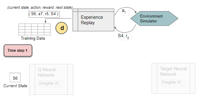
The sample data (Current state, action, reward, next state) is saved
Experience Replay executes the ε-greedy action and receives the next state and reward.
It stores the results in the replay data. Each such result is a sample observation which will later be used as training data.
 (Image by Author)
Select random training batch
We now start the phase to train the DQN. Select a training batch of random samples from the replay data as input for both networks.
 (Image by Author)
Use the current state from the sample as input to predict the Q values for all actions
To simplify the explanation, let’s follow a single sample from the batch. The Q network predicts Q values for all actions that can be taken from the state.
 (Image by Author)
Select the Predicted Q-value
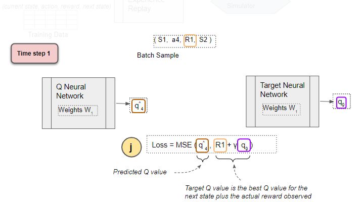
From the output Q values, select the one for the sample action. This is the Predicted Q Value.
 (Image by Author)
Use the next state from the sample as input to the Target network
The next state from the sample is input to the Target network. The Target network predicts Q values for all actions that can be taken from the next state, and selects the maximum of those Q values.
Use the next state as input to predict the Q values for all actions. The target network selects the max of all those Q-values.
 (Image by Author)
Get the Target Q Value
The Target Q Value is the output of the Target Network plus the reward from the sample.
 (Image by Author)
Compute Loss
Compute the Mean Squared Error loss using the difference between the Target Q Value and the Predicted Q Value.
 (Image by Author)
Compute Loss
 (Image by Author)
Back-propagate Loss to Q-Network
Back-propagate the loss and update the weights of the Q Network using gradient descent. The Target network is not trained and remains fixed, so no Loss is computed, and back-propagation is not done. This completes the processing for this time-step.
 (Image by Author)
No Loss for Target Network
The Target network is not trained so no Loss is computed, and back-propagation is not done.
Repeat for next time-step
The processing repeats for the next time-step. The Q network weights have been updated but not the Target network’s. This allows the Q network to learn to predict more accurate Q values, while the target Q values remain fixed for a while, so we are not chasing a moving target.
 (Image by Author)
After T time-steps, copy Q Network weights to Target Network
After T time-steps, copy the Q network weights to the Target network. This lets the Target network get the improved weights so that it can also predict more accurate Q values. Processing continues as before.
 (Image by Author)
The Q network weights and the Target network are again equal.
Conclusion
In the previous article, we had seen that Q-Learning used the Target Q Value, the Current Q Value, and observed reward to update the Current Q Value using its update equation.
The DQN works in a similar way. Since it is a neural network, it uses a Loss function rather than an equation. It also uses the Predicted (ie. Current) Q Value, Target Q Value, and observed reward to compute the Loss to train the network, and thus improve its predictions.
In the next article, we will continue our Deep Reinforcement Learning journey, and look at another popular algorithm using Policy Gradients.
And finally, if you liked this article, you might also enjoy my other series on Transformers as well as Audio Deep Learning.
Transformers Explained Visually - Overview of functionality
Audio Deep Learning Made Simple - State-of-the-Art Techniques
Let’s keep learning!