Reinforcement Learning Made Simple - Solution Approaches

This is the second article in my series on Reinforcement Learning (RL). Now that we understand what an RL Problem is, let’s look at the approaches used to solve it.

Here’s a quick summary of the previous and following articles in the series. My goal throughout will be to understand not just how something works but why it works that way.

1. Intro to Basic Concepts and Terminology (What is an RL problem, and how to apply an RL problem-solving framework to it using techniques from Markov Decision Processes and concepts such as Return, Value, and Policy)
2. Solution Approaches — this article (Overview of popular RL solutions, and categorizing them based on the relationship between these solutions. Important takeaways from the Bellman equation, which is the foundation for all RL algorithms.)
3. Model-free algorithms (Similarities and differences of Value-based and Policy-based solutions using an iterative algorithm to incrementally improve predictions. Exploitation, Exploration, and ε-greedy policies.)
4. Q-Learning (In-depth analysis of this algorithm, which is the basis for subsequent deep-learning approaches. Develop intuition about why this algorithm converges to the optimal values.)
5. Deep Q Networks (Our first deep-learning algorithm. A step-by-step walkthrough of exactly how it works, and why those architectural choices were made.)
6. Policy Gradient (Our first policy-based deep-learning algorithm.)
7. Actor-Critic (Sophisticated deep-learning algorithm which combines the best of Deep Q Networks and Policy Gradients.)

RL Solution Categories

‘Solving’ a Reinforcement Learning problem basically amounts to finding the Optimal Policy (or Optimal Value). There are many algorithms, which we can group into different categories.

Model-based vs Model-free

Very broadly, solutions are either:

• Model-based (aka Planning)
• Model-free (aka Reinforcement Learning)

Model-based approaches are used when the internal operation of the environment is known. In other words, we can reliably say what Next State and Reward will be output by the environment when some Action is performed from some Current State.

Model-based: Internal operation of the environment is known (Image by Author)

Model-free approaches are used when the environment is very complex and its internal dynamics are not known. They treat the environment as a black-box.

Model-free: Environment is a black box (Image by Author)

Prediction vs Control

Another high-level distinction is between Prediction and Control.

With a Prediction problem, we are given a Policy as input, and the goal is to output the corresponding Value function. This could be any Policy, not necessarily an Optimal Policy.

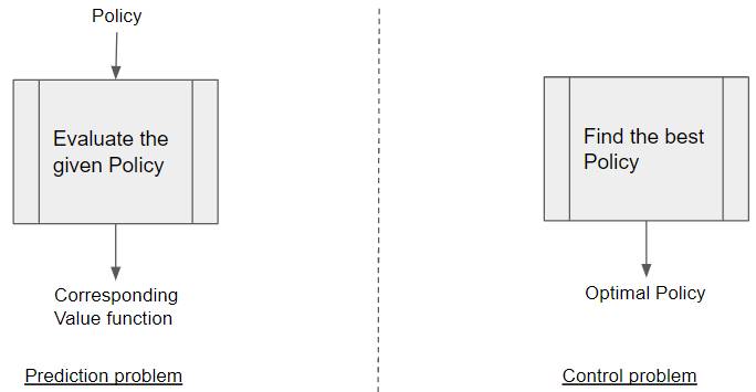Prediction vs Control problems (Image by Author)

With a Control problem, no input is provided, and the goal is to explore the policy space and find the Optimal Policy.

Most practical problems are Control problems, as our goal is to find the Optimal Policy.

Classifying Popular RL Algorithms

The most common RL Algorithms can be categorized as below:

Taxonomy of well-known RL Solutions (Image by Author)

Most interesting real-world RL problems are model-free control problems. So we will not explore model-based solutions further in this series other than briefly touching on them below. Everything we discuss from here on pertains only to model-free control solutions.

Model-based Approaches

Because they can produce the exact outcome of every state and action interaction, model-based approaches can find a solution analytically without actually interacting with the environment.

As an example, with a model-based approach to play chess, you would program in all the rules and strategies of the game of chess. On the other hand, a model-free algorithm would know nothing about the game of chess itself. Its only knowledge would be generic information such as how states are represented and what actions are possible. It learns about chess only in an abstract sense by observing what reward it obtains when it tries some action.

Most real-world problems are model-free because the environment is usually too complex to build a model.

Model-free Approaches

Model-free solutions, by contrast, are able to observe the environment’s behavior only by actually interacting with it.

Interact with the environment

Since the internal operation of the environment is invisible to us, how does the model-free algorithm observe the environment’s behavior?

We learn how it behaves by interacting with it, one action at a time. The algorithm acts as the agent, takes an action, observes the next state and reward, and repeats.

Model-free algorithms learn about the environment by interacting with it, one action at a time. (Image by Author)

The agent acquires experience through trial and error. It tries steps and receives positive or negative feedback. This is much the same as a human would learn.

Trajectory of interactions

As the agent takes each step, it follows a path (ie. trajectory).

A trajectory of interactions (Image by Author)

The agent’s trajectory becomes the algorithm’s ‘training data’.

The Bellman Equation is the foundation for all RL algorithms

Before we get into the algorithms used to solve RL problems, we need a little bit of math to make these concepts more precise.

The math is actually quite intuitive — it is all based on one simple relationship known as the Bellman Equation.

This relationship is the foundation for all the RL algorithms. This equation has several forms, but they are all based on the same basic idea. Let’s go through this step-by-step to build up the intuition for it.

Work back from a Terminal State (makes it easier to understand)

Consider the reward by taking an action from a state to reach a terminal state.

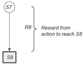Reward when reaching a terminal state (Image by Author)

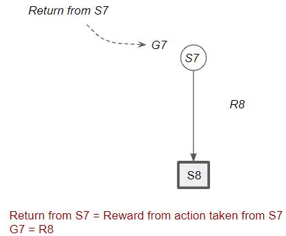
The return from that state is the same as the reward obtained by taking that action. Remember that Reward is obtained for a single action, while Return is the cumulative discounted reward obtained from that state onward (till the end of the episode).

(Image by Author)

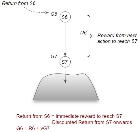
Now consider the previous state S6. The return from S6 is the reward obtained by taking the action to reach S7 plus any discounted return that we would obtain from S7. The important thing is that we no longer need to know the details of the individual steps taken beyond S7.

(Image by Author)

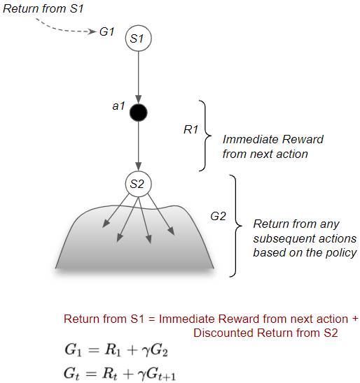
Bellman Equation for Return

In general, the return from any state can be decomposed into two parts — the immediate reward from the action to reach the next state, plus the Discounted Return from that next state by following the same policy for all subsequent steps. This recursive relationship is known as the Bellman Equation.

(Image by Author)

Bellman Equation for State Value

Return is the discounted reward for a single path. State Value is obtained by taking the average of the Return over many paths (ie. the Expectation of the Return).

So State Value can be similarly decomposed into two parts — the immediate reward from the next action to reach the next state, plus the Discounted Value of that next state by following the policy for all subsequent steps.

(Image by Author)

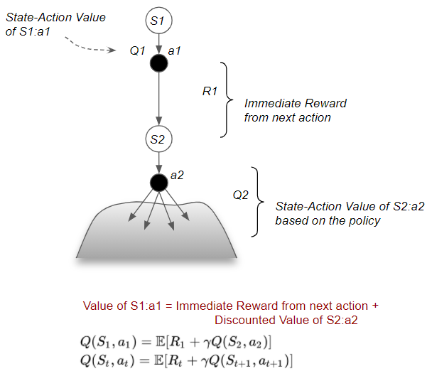
Bellman Equation for State-Action Value

Similarly, the State-Action Value can be decomposed into two parts — the immediate reward from that action to reach the next state, plus the Discounted Value of that next state by following the policy for all subsequent steps.

(Image by Author)

Why is the Bellman Equation useful?

There are two key observations that we can make from the Bellman Equation.

Return can be computed recursively without going to the end of the episode

The first point is that, in order to compute the Return, we don’t have to go all the way to the end of the episode. Episodes can be very long (and expensive to traverse), or they could be never-ending. Instead, we can use this recursive relationship.

If we know the Return from the next step, then we can piggy-back on that. We can take just a single step, observe that reward, and then re-use the subsequent Return without traversing the whole episode beyond that.

We can work with estimates, rather than exact values

The second point is that there are two ways to compute the same thing:

• One is the Return from the current state.
• Second is the reward from one step plus the Return from the next state.

Why does this matter?

Since it is very expensive to measure the actual Return from some state (to the end of the episode), we will instead use estimated Returns. Then we compute these estimates in two ways and check how correct our estimates are by comparing the two results.

Since these are estimates and not exact measurements, the results from those two computations may not be equal. The difference tells us how much ‘error’ we made in our estimates. This helps us improve our estimates by revising them in a way that reduces that error.

Hang on to both these ideas because all the RL algorithms will make use of them.

Conclusion

Now that we have an overall idea about what an RL problem is, and the broad landscape of approaches used to solve them, we are ready to go deeper into the techniques used to solve them. Since real-world problems are most commonly tackled with model-free approaches, that is what we will focus on. They will be the topic of the next article.

And finally, if you liked this article, you might also enjoy my other series on Transformers as well as Audio Deep Learning.

Transformers Explained Visually - Overview of functionality

Audio Deep Learning Made Simple - State-of-the-Art Techniques

Let’s keep learning!