
This is the third article in my series on Reinforcement Learning (RL). Now that we understand what an RL Problem is, and the types of solutions available, we’ll now learn about the core techniques used by all solutions.
Using an iterative algorithm as a framework to incrementally improve predictions, we’ll understand the fundamental similarities and differences between Value-based and Policy-based solutions.
Here’s a quick summary of the previous and following articles in the series. My goal throughout will be to understand not just how something works but why it works that way.
- Intro to Basic Concepts and Terminology (What is an RL problem, and how to apply an RL problem-solving framework to it using techniques from Markov Decision Processes and concepts such as Return, Value, and Policy)
- Solution Approaches (Overview of popular RL solutions, and categorizing them based on the relationship between these solutions. Important takeaways from the Bellman equation, which is the foundation for all RL algorithms.)
- Model-free algorithms — this article (Similarities and differences of Value-based and Policy-based solutions using an iterative algorithm to incrementally improve predictions. Exploitation, Exploration, and ε-greedy policies.)
- Q-Learning (In-depth analysis of this algorithm, which is the basis for subsequent deep-learning approaches. Develop intuition about why this algorithm converges to the optimal values.)
- Deep Q Networks (Our first deep-learning algorithm. A step-by-step walkthrough of exactly how it works, and why those architectural choices were made.)
- Policy Gradient (Our first policy-based deep-learning algorithm.)
- Actor-Critic (Sophisticated deep-learning algorithm which combines the best of Deep Q Networks and Policy Gradients.)
Model-free algorithms can be Policy-based or Value-based
Use the Value function to compare two policies
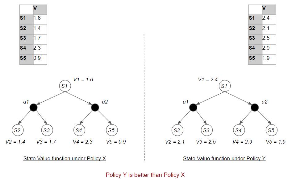
As we discussed in the first article, every policy has two corresponding value functions, the State Value (or V-value), and the State-Action Value (or Q-value), and that we can use a policy’s value functions to compare two policies. Policy Y is ‘better’ than Policy X if Y’s value function is ‘higher’ than X’s.
 Compare Policies by comparing their respective Value functions (Image by Author)
Optimal Policy
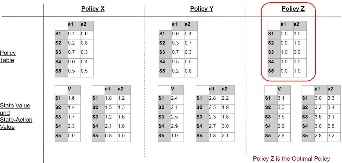
We had also discussed that if we keep finding better and better policies, we will eventually be able to find the ‘best’ policy which is better than all other policies. This is the Optimal Policy.
 Optimal Policy is better than all other policies (Image by Author)
Optimal Policy goes hand-in-hand with Optimal Value
The Optimal Policy has two corresponding value functions. By definition, those value functions are better than all other value functions. Hence those value functions are also optimal ie. the Optimal State Value and Optimal State-Action Value.
 The value functions corresponding to the Optimal Policy are the Optimal Value functions. (Image by Author)
This tells us that finding an Optimal Policy is equivalent to finding the Optimal State-Action Value, and vice versa. By finding one we also get the other, as we see below.
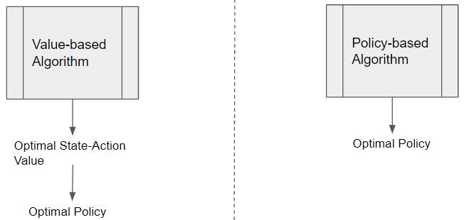
Policy-based vs Value-based algorithms
Consequently, model-free algorithms can find the Optimal Policy directly or indirectly. They are either:
- State-Action Value-based (indirect). For brevity, we will refer to these as simply “Value-based”
- Policy-based (direct)
 Model-free solutions find the Optimal Policy directly or indirectly (Image by Author)
Value-based algorithms find the Optimal State-Action Value. The Optimal Policy can then be derived from it. Policy-based algorithms don’t need the Optimal Value and find the Optimal Policy directly.
Derive the Optimal Policy from the Optimal State-Action Value
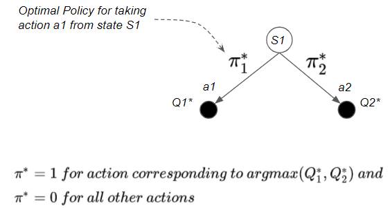
Once a Value-based algorithm finds the Optimal State-Action Value, how does it find the Optimal Policy from it?
Once we find the Optimal State-Action Value, we can easily obtain the Optimal Policy by picking the action with the highest State-Action value.
 We can obtain the Optimal Policy from the Optimal State-Action Value (Image by Author)
Consider the example above. If Q1* > Q2*, then the Optimal Policy will pick action a1 in state S1.
Hence, π1* = 1 and π2* = 0
This gives us a deterministic Optimal Policy
Generally, the Optimal Policy is deterministic since it always picks the best action.
However, the Optimal Policy could be stochastic if there is a tie between two Q-values. In that case, the Optimal Policy picks either of the two corresponding actions with equal probability. This is often the case for problems where the agent plays a game against an opponent. A stochastic Optimal Policy is necessary because a deterministic policy would result in the agent playing predictable moves that its opponent could easily defeat.
State-Value-based algorithms for Prediction problems
In addition to the State-Action Value-based algorithms mentioned above, which are used for solving Control problems, we also have State-Value-based algorithms, which are used for Prediction problems. In other words:
- Prediction algorithms are State-Value based
- Control algorithms are either State-Action Value-based or Policy-based
Model-free Algorithm Categories
Lookup Table vs Function
Simpler algorithms implement the Policy or Value as a Lookup Table, while the more advanced algorithms implement a Policy or Value function, using a Function Approximator like a Neural Network.
We can thus group model-free algorithms into categories as below:
 (Image by Author)
Model-free algorithms use an iterative solution
The RL problem cannot be solved algebraically. We need to use an iterative algorithm.
There are several such Value-based and Policy-based algorithms. I found it quite bewildering at first when I started to dive into the specifics of each of those algorithms. However, after a while, I began to realize that all of these algorithms can be boiled down to a few essential principles that all of them employ.
So, instead, if we focus on learning what those principles are, it will make it very easy to understand how these algorithms relate to one another and what their similarities and differences are.
And then, when we go into the details of each algorithm in later articles, you will be able to quickly see how these common principles are being applied, without getting lost.
At a high-level, all algorithms, both Value-based and Policy-based, have four basic operations that they perform. They start with arbitrary estimates of the quantity they want to find, and then incrementally improve those estimates by getting data from the environment.
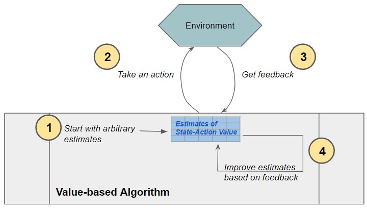 Value-based algorithm (as well as Policy-based) perform these four basic operations. (Image by Author)
Let’s look at each of these four operations and compare Value-based and Policy-based approaches.
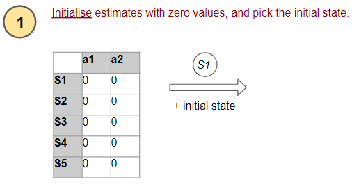
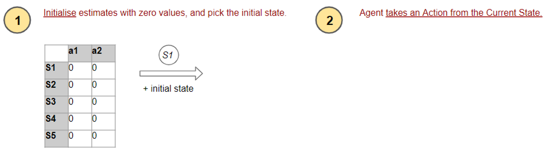
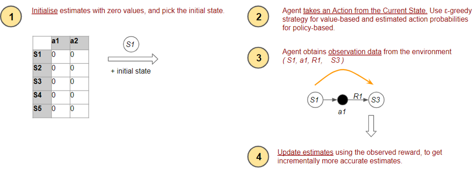
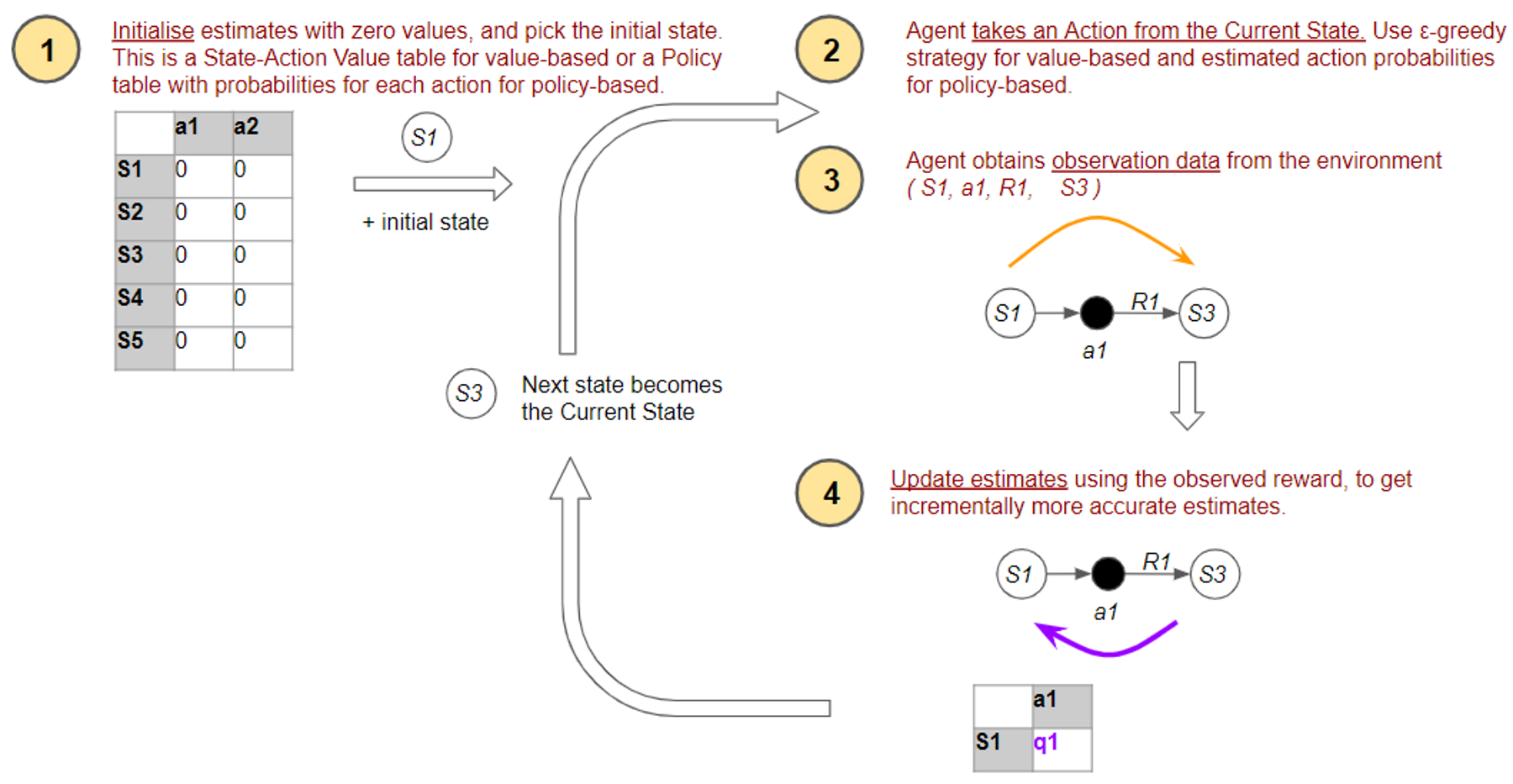
1. Initialize estimates
The first step is the Initialization of our estimates. A Value-based algorithm uses an estimated Optimal State-Action Value table, while a Policy-based algorithm uses an estimated Optimal Policy table with probabilities for each action in each state.
 (Image by Author)
In the beginning, since it has no idea what the right values are, it simply initializes everything to zero.
2. Take an action
Next, the agent needs to pick an action to perform from the current state.
 (Image by Author)
The agent wants to ensure that it tries all the available paths sufficiently so that it discover the best ones, and doesn’t miss out on the best options. How does it do this?
 (Image by Author)
To solve this we need to understand the concept of Exploration and Exploitation.
Exploration vs Exploitation
Exploration — when we first start learning, we have no idea which actions are ‘good’ and which are ‘bad. So we go through a process of discovery where we randomly try different actions and observe the rewards.
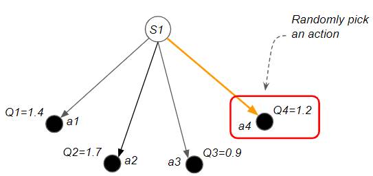 Exploration: Discover new paths by randomly picking an action (Image by Author)
Exploitation — on the other end of the spectrum, when the model is fully trained, we have already explored all possible actions, so we can pick the best actions which will yield the maximum return
 Exploitation: Pick the best action to maximize return (Image by Author)
The agent needs to find the right balance between Exploration and Exploitation. Policy-based agents and Value-based agents use different methods to achieve this.
Policy-based uses its own estimates to pick an action
A Policy-based agent’s Policy Table already has an ongoing estimate of the optimal policy, which tells you the desired probability of all the actions you can take from any given state. So it just picks an action based on the probabilities of that estimated optimal policy. The higher the probability of an action, the more likely it is to get picked.
 A policy-based approach to pick the best action (Image by Author)
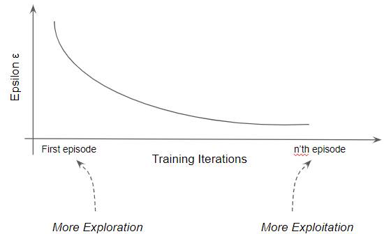
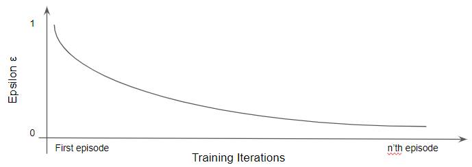
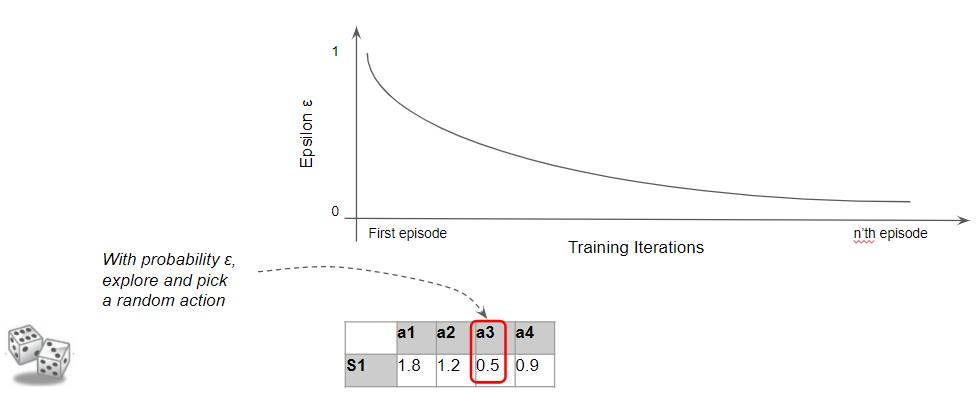
Value-based uses an ε-greedy strategy to pick an action
A Value-based agent adopts a dynamic strategy known as ε-Greedy. It uses an exploration rate ε which it adjusts as training progresses to ensure more exploration in the early stages of training and shifts towards more exploitation in the later stages.
 A value-based approach uses an ε-greedy strategy (Image by Author)
We set ε initially to 1. Then, at the start of each episode, we decay ε by some rate.
 (Image by Author)
Now, whenever it picks an action in every state, it selects a random action (ie. explores) with probability ε. Since ε is higher in the early stages, the agent is more likely to explore.
 (Image by Author)
And similarly, with probability ‘1 — ε’, it selects the best action (ie. exploit). As ε goes down, the likelihood of exploration becomes less and the agent becomes ‘greedy’ by exploiting the environment more and more.
 (Image by Author)
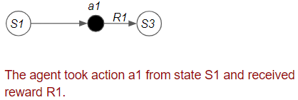
3. Get feedback from the environment
The agent takes the action it has selected and obtains feedback from the environment.
 (Image by Author)
The agent receives feedback from the environment in the form of a reward.
 (Image by Author)
4. Improve estimates
How does the agent use the reward to update its estimates so that they become more accurate?
 (Image by Author)
A Policy-based agent uses that feedback to improve its estimated Optimal Policy based on that reward. A Value-based agent uses that feedback to improve its estimated Optimal Value based on that reward. That way, the next time they have to decide which action to take from that state, that decision will be based on more accurate estimates.
Policy-based updates the probability of the action
The agent says ‘If I got a positive reward, then I will update my Policy table to increase the probability of the action I just took. That way, the next time I will be more likely to take that action’
 (Image by Author)
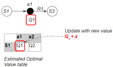
Value-based updates its value based on the Bellman Equation
A Value-based agent says ‘My previous estimate told me to expect this much Value from this action. Based on the reward I just got, the Bellman Equation tells me that my Value should be higher (or lower). I will update my Value table to reduce that gap.’
 (Image by Author)
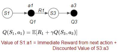
We’ll go deeper into how the value-based agent uses the Bellman Equation to improve its estimates. We discussed the Bellman Equation in-depth in the second second article, so it might be a good idea to go back and refer to it as a refresher.
That equation describes a recursive relationship to calculate the Q-value. The first important insight from this is that, if we know the Q-value of the next state-action pair, then we can piggy-back on it, without having to traverse the whole episode beyond that.
 (Image by Author)
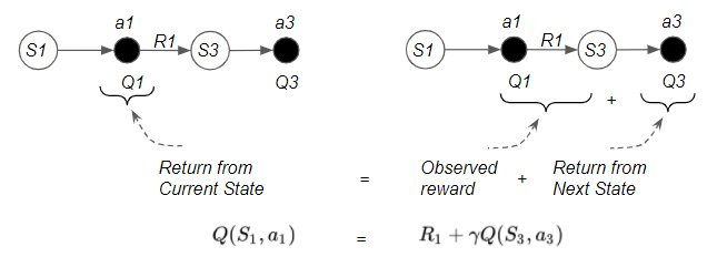
The second important insight is that the Bellman Equation says that there are two ways to compute the State-Action Value:
- One way is the State-Action Value from the Current State
- The other way is the immediate reward from taking one step plus the State-Action Value from the Next State
 (Image by Author)
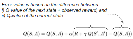
This tells us that we can obtain the State Value in two different ways. If these were perfectly accurate values, these two quantities would be exactly equal.
However, since the algorithm is using estimated values, we can check whether our estimates are correct by comparing those two quantities.
If they are not equal, the ‘difference’ tells us the amount of ‘error’ in our estimates.
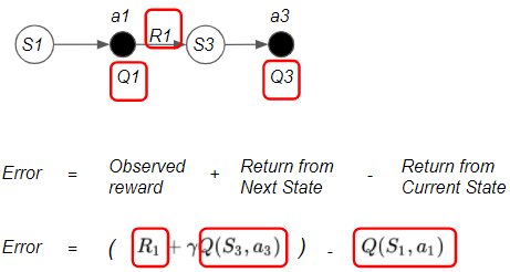 (Image by Author)
The first term contains an actual reward plus an estimate, while the second term is only an estimate.
The algorithm incrementally updates its Q-value estimates in a way that reduces the error.
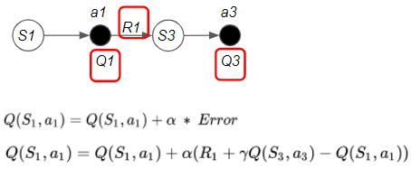 (Image by Author)
Putting it all together
The agent now has improved estimates. This completes the flow for the four operations. The algorithm continues doing this flow till the end of the episode. Then it restarts a new episode and repeats.
 (Image by Author)
Different Ways to Improve Estimates
The core of the algorithm is how it improves its estimates. Different algorithms use slightly different techniques for doing this. These variations are mainly related to three factors:
- Frequency — the number of forward steps taken before an update.
- Depth — the number of backward steps to propagate an update.
- Formula that is used to compute the updated estimate.
Let’s briefly go over these factors to get a flavor of what these variations are.
Frequency
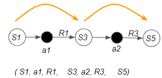
There are three options for the number of forward steps the agent can take before updating our estimates:
- Episode — The simplest idea is that it takes an action, observes rewards, saves them, then takes another action, observes those rewards and saves them, and keeps doing that till the end of the episode. Finally, at the end of the episode, the algorithm takes all those rewards and uses them to update our estimates.
- One Step — Alternately, rather than waiting till we go all the way to the end of the episode, we could take just one step, observe those rewards and do the update right away.
- N Steps — The above two options are the two ends of the spectrum. In between, we could do the update after N steps.
 (Image by Author)
In the general case, the agent takes some forward steps. This could be one step, N steps, or till the end of the episode.
Depth
After taking some forward steps, the next question is how far back should the algorithm propagate its update estimates? Again, there are three options:
- Episode — If the agent took forward steps till the end of the episode, the algorithm could update the estimates for every state-action pair that it took along the way.
- One Step — Alternately, it could update the estimates for only the current state-action pair.
- N Steps — The above two options are the two ends of the spectrum. In between, we could update N steps along the way
 (Image by Author)
After taking some forward steps, the algorithm updates estimates for the states and actions it took. This could be a single step for the current state-action pair, N steps, or till the beginning of the episode.
Update Formula
The formula used to update the estimates has many variations eg:
- Value-based updates use some flavor of the Bellman Equation to update the Q-value with an ‘error’ value. For example, this formula incrementally updates the Q-value estimate with an error value known as the TD Error.
 (Image by Author)
- Policy-based updates increase or decrease the probability of the action that the agent took, based on whether we received a good reward or not.
Relationship between Model-free Algorithms
If you study the different algorithms, each one seems very different. However, as we’ve just seen, there are some similar patterns that they all follow.
In this series, we will not go into every one of these algorithms but will focus on the few which are popularly used in deep reinforcement learning.
However, just for completeness, I’ve put together a table that summarizes the relationship between these algorithms. It helped make things a lot clearer to me when I was learning about them. So I hope you find it helpful as well.
 (Image by Author)
Conclusion
In this article, we got an overview of solutions for RL problems and explored the common themes and techniques used by some popular algorithms. We focused primarily on Model-free Control algorithms which are used to solve most real-world problems.
We are now ready to dive into the details of the neural-network-based deep learning algorithms. They are the ones of most interest, as they have made tremendous strides in addressing complex and previously intractable problems in the last few years.
We will pick one algorithm in each of the next few articles, starting with Q Learning which is the foundation for the deep learning algorithms.
And finally, if you liked this article, you might also enjoy my other series on Transformers as well as Audio Deep Learning.
Transformers Explained Visually - Overview of functionality
Audio Deep Learning Made Simple - State-of-the-Art Techniques
Let’s keep learning!